Team passing styles in Allsvenskan 2021
Short or long? Slow build-up or fast counter attack? Central or wide? These are all questions you may ask yourself when trying to describe how a team plays football. Can we find out the answers to (some of) these questions by analyzing passes made by each team?
Following my previous post on detecting player passing style, let us now shed light on how the the passing styles varied among the teams in Allsvenskan 2021 by clustering.
Introduction
No action is as prevalent in the game of football as the pass, whether it be a short pass between center-backs or an attempt at a crucial through ball to send the striker through on goal. It has been found that approximately 65% of all actions are passes [1]. As it is by far the most common action in football, passes represent a crucial component of a team’s playing style. When watching games we can see how different teams structure their possession in various ways. Can we also find similar patterns from data analysis of passing play? Join me in finding out the answer to this question!
For the code of this analysis, refer to this Github repo.
Data
The data originates from the open data repository of PlaymakerAI and without it, the rest of this work would not be possible.
As for the data used for the analysis, it contains all games in Allsvenskan during the 2021 season. Each game consists of approximately 1200-1500 actions that describe the events that take place during a game, e.g., passes, shots, tackles etc. Furthermore, each action is also described by what (the action taking place), who (the player and team performing the action), where (start and end $x$ and $y$ coordinates), and when (start and end time).
Pitch plot
To give a feeling of where the actions take place, refer to the following figure:
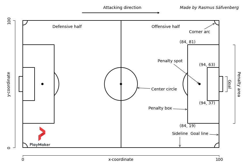
where each team always attacks left to right.
Selecting passing variables
From the data, the first step was to determine which passing variables could be derived and analyzed. The following variables were included:
| Variable | Description | Length | Outcome |
|---|---|---|---|
| Assist | Pass leading to goal. | Long/Medium/Short | Success |
| Cross | Pass from the wing to the central attacking third. | Long/Medium/Short | Success/Fail |
| Final third entry | Pass from outside that enters the final third. | Long/Medium/Short | Success/Fail |
| Key pass | Pass leading to a shot or goal scoring opportunity. | Long/Medium/Short | Success |
| Pass into the box | A pass that ends inside the penalty box. | Long/Medium/Short | Success/Fail |
| Pass | All passes, with the exception of goal kicks. | Long/Medium/Short | Success/Fail |
| Progressive pass | According to the Wyscout definition. | Long/Medium/Short | Success/Fail |
| Wing switch | A pass going from wing to wing, at least half the pitch width. | Long/Medium | Success/Fail |
Variables regarding corners and clearances were excluded due to the corners not being in open play and clearances not always being a pass, as well as lacking end coordinates.
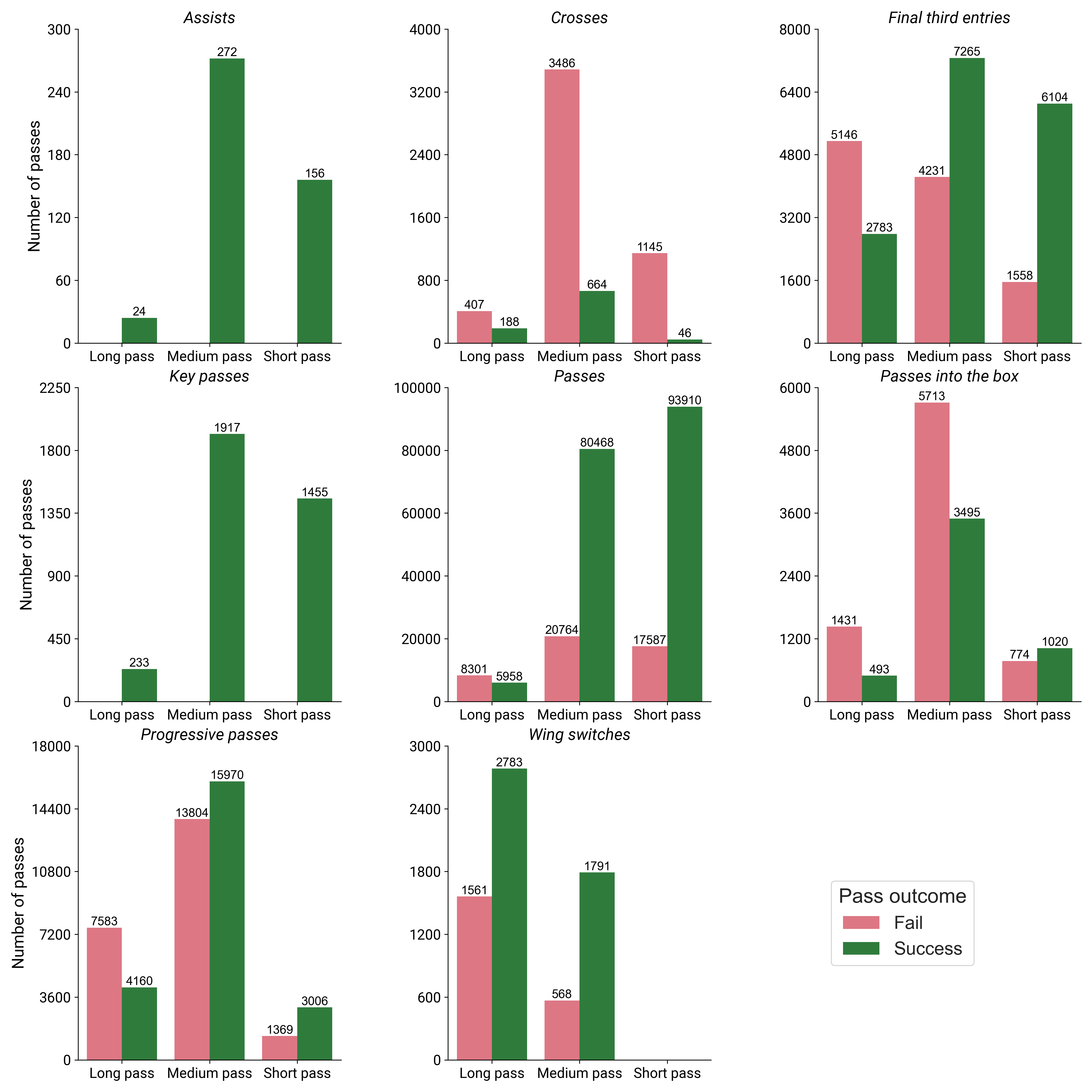
Exploring passing variables
Prior to the analysis, we can as a first step investigate the number of passes per category as well as their rate of success. The counts given are total for all teams and games across the entire season. Also note the fact that they y-axes are different for each plot.
Preprocessing
After retrieving the data the next step is to process it such that an analysis can be performed. In particular, the data should be transformed from long to wide.
Data in long format is characterized by multiple rows describing the same action, e.g., a pass that is also a cross would therefore span two rows, one for the pass and another for the cross. However, for the analysis that will follow, the data should be in wide format, where each row describes a unique action. In the wide representation, each action will therefore be represented by the most succinct action, where in the previous example the pass would be be described as a cross (as a cross is also a pass, but the opposite need not be true).
Although, this is the general procedure, some actions are not kept in the same way. These actions are assists, key passes, and passes into the box. This is due to the basis for the analysis being founded on the SPADL definition from [1].
Further preprocessing steps include:
- Create a separate column containing the result of each action (success/fail).
- Adding boolean columns for key passes, assists, and passed into the box to indicate whether the pass also has one of the additional tags.
- Transforming the pitch coordinates to $x \in [0, 105]$ and $y \in [0, 68]$.
- Computing the distance of passes.
- Determining if a pass was a progressive pass or not.
- Adding a column for the passing length, which is defined as:
- short, if the pass distance is less than 15 meters, or
- medium, if the pass distance is between 15 and 40 meters, or
- long, if the pass distance exceeds 40 meters.
- Computing the number of passes per result and pass length for each player in each game.
- Note that goal kicks and goalkeeper throws are excluded in this step.
- The player's value is then divided by the minutes played in the game.
- And in turn, the value is then also divided by the possession his team had in the game.
- Next, the value is multiplied by 90 to represent the count per 90 minutes.
- In this step we also filter out players who played less than 300 minutes during the season.
- After computing these standardized statistics, the next step is sum the to be for the entire season.
- Finally, before feeding the data to the next step, we normalize the data by subtracting the mean and scale to unit variance. This ensures the variables are all on the same scale.
Note: The keen reader will notice that a possession adjustment of the passing statistics is performed and might wonder why. The reason for such a choice is two-fold. One, it is not uncommon for a few teams to be more possession oriented and thus make more passes per game. This may skew things in their favor as they simply have more passes than their opposition. Second, I am more interested in what they do with the ball, rather than if they control it for extended periods of time. Consequently, we will be looking at how each team passes in a league where they all have an equal share of possession.
Whew! That was a “short” summary of the preprocessing! If you would like to check the preprocessing in detail, check out the scripts in the Github repo.
Method
Prior to examining the results, we should go through how we obtain said results. But first, let’s quickly define some terms to make sure we are on the same page.
- Data
- The data is in this case a matrix of $n=16$ rows (=teams) and $p=40$ variables, which will also be referred to as dimensions.
- Dimensionality reduction
- Transforming data from many dimensions to fewer, while maintaining as much information as possible.
- Cluster
- A grouping of objects that are similar.
- Clustering
- The method of assigning grouping objects together into cohesive clusters.
Reducing the dimensionality of the data
Similarly to my previous post, we again have data with a higher dimensionality. Specifically, we have 40 variables in total, which arises from the combination of pass type, pass length and pass outcome. As a result, we will yet again leverage principal component analysis (PCA).
PCA is a method to capture most of the information in the data, but with fewer dimensions. This is accomplished by creating linear combinations (=components) of the original variables by maximizing the (orthogonal) variance in a given direction. That is, the first dimension explains the most variance, the second dimension has the second most variance explained and so on. This is then transformed into a new coordinate system.
Each principal component also consists of a set of loadings, which refers to the coefficient of each original variable. That is, how much each variable impacts a given principal component. After fitting PCA we can then transform the original variables into the corresponding PCA coordinate system. Yet again, we use parallel analysis1 to decide on the number of components to retain, which resulted in only the first two components being retained. The reason for doing PCA in the first place is that the concept of distance can become obtuse in higher dimension and this could be problematic for the upcoming clustering.
Hierarchical clustering
After transforming the data into PCA space, we can look into how to actually group the different teams. Recall that a cluster is just a statistical term for group. Since our set of teams is quite small ($n=16$), we can investigate hierarchical clustering. Hierarchical clustering aims to perform clustering by forming clusters that are hiearchically linked to each other. In general, there are two different types of hierarchical clustering: agglomerative and divisive (yes, statisticians and mathematicians like long and fancy words). The difference is, however, quite simple.
Agglomerative clustering works by letting each
observation (=team) start out as its own cluster and we then pair them together as we progress
through the hierarchy.
Divisive clustering is the opposite, by starting with one big
cluster and then separating into smaller clusters (recursively). An example of this
will be seen in the result section.
Here we will use hierarchical agglomerative clustering, and the choice of algorithm is based on a mixture of data size2 and ability to interpret the results. Before moving on, we also need to discuss the concept of linkage. In this context, a linkage refers to the process of computing the distance $d$ between two clusters $c_1$ and $c_2$ and how to combine them. Initially, we begin with all (individual) clusters that are yet to be merged with one another. Then we find the two clusters that are closest to each other and merge them into a new cluster, say $c^{(1)}$, where the clusters $c_1$ and $c_2$ are then removed from the set of clusters, instead replaced by the newly formed cluster. This is then repeated until only one cluster remains, which will contain all observations, and this final cluster is then seen as the start (=root) of the clustering. Typically, this type of clustering can be described by using a tree analogy, where we are moving from the leafs (individual clusters), along the branches (merged clusters) all the way until the root (final cluster with all observations). As with most algorithms, there are some choices to be made regarding what linkage method should be chosen. Common choices include single, average, complete, and Ward linkage. For this analysis, the choice is Ward linkage3, which aims at (incrementally) minimizing the variance when deciding which cluster(s) to form.
Results
Moving swiftly onwards, let us now examine the results.
Dimensionality reduction
First of all, we can see how much of the total variance in the data is explained by each principal component to get a feel for the transformation.
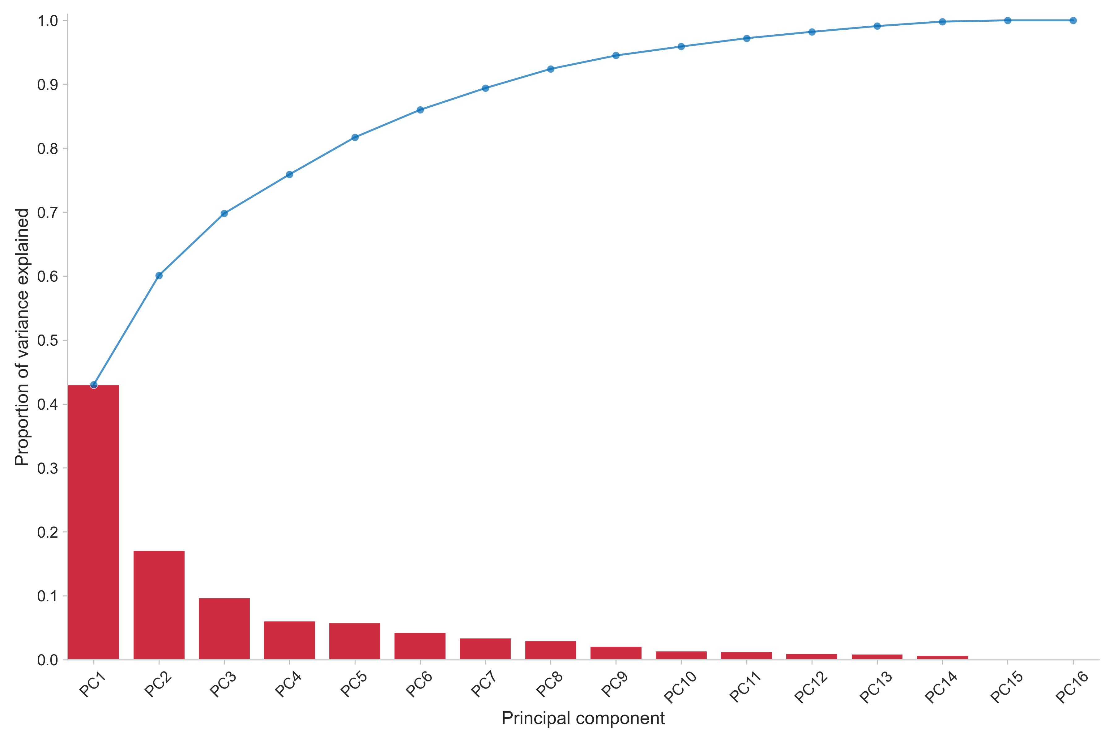
Here we can see that the first two components explain approximately 60 % together, where the first is responsible for slightly above 40 %. The following components all explain 10 % or less of the variance. A reminder is that it was suggested by parallel analysis to only retain the first two components.
Next, we investigate how the magnitude of passing variables on the components via their loadings.

As the green values indicate a positive coefficient, while red is the opposite, we can observe that the first component has coefficients close to one for successful short and medium passing. Moreover, it has negative weights for all long passing variables. For the second component, long passing instead has some negative and some positive loadings but the positive loadings are given to the failed passes. A negative loading can also be found for successful key passes, final third entries, and passes into the box.
Based on these loadings and the fact we have can visualize the first two principal components, we can summarize this information in a scatter plot prior to fitting the clustering.
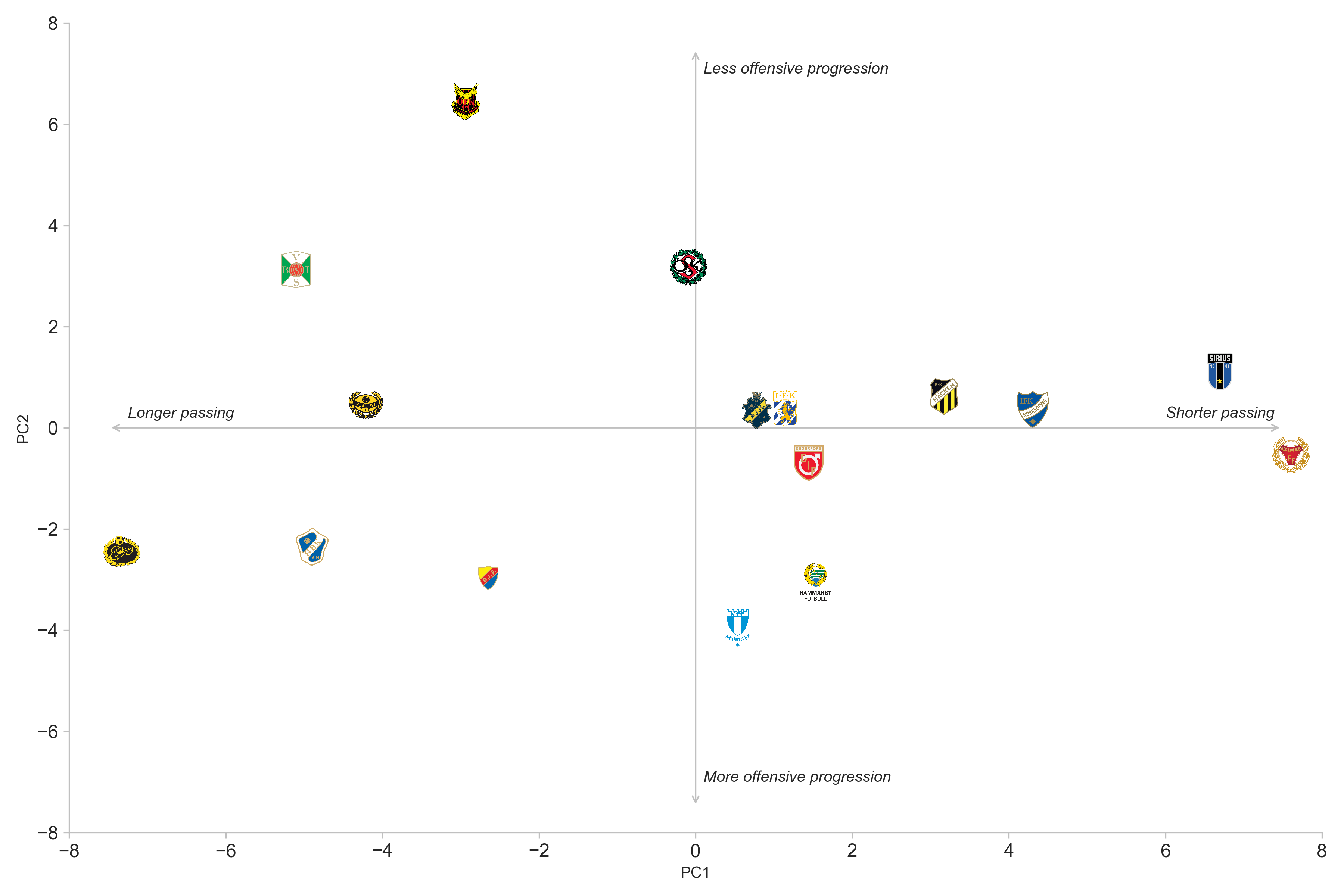
The figure shows an indication of what we can expect in the clustering. One such indication is that a split between long and short passing will probably be found, as well as a distinction between teams that have more offensive progression. From this graph, it seems that AIK and IFK Göteborg are the most similar teams. The arrows in the plot also gives a simplified description of the how the passing styles varies by team.
Reminder: All passing statistics are possession-adjusted.
Clustering
Moving forward, let us now turn our attention to the clustering: the meat and bones of this analysis. Let us start by fitting an initial HAC.
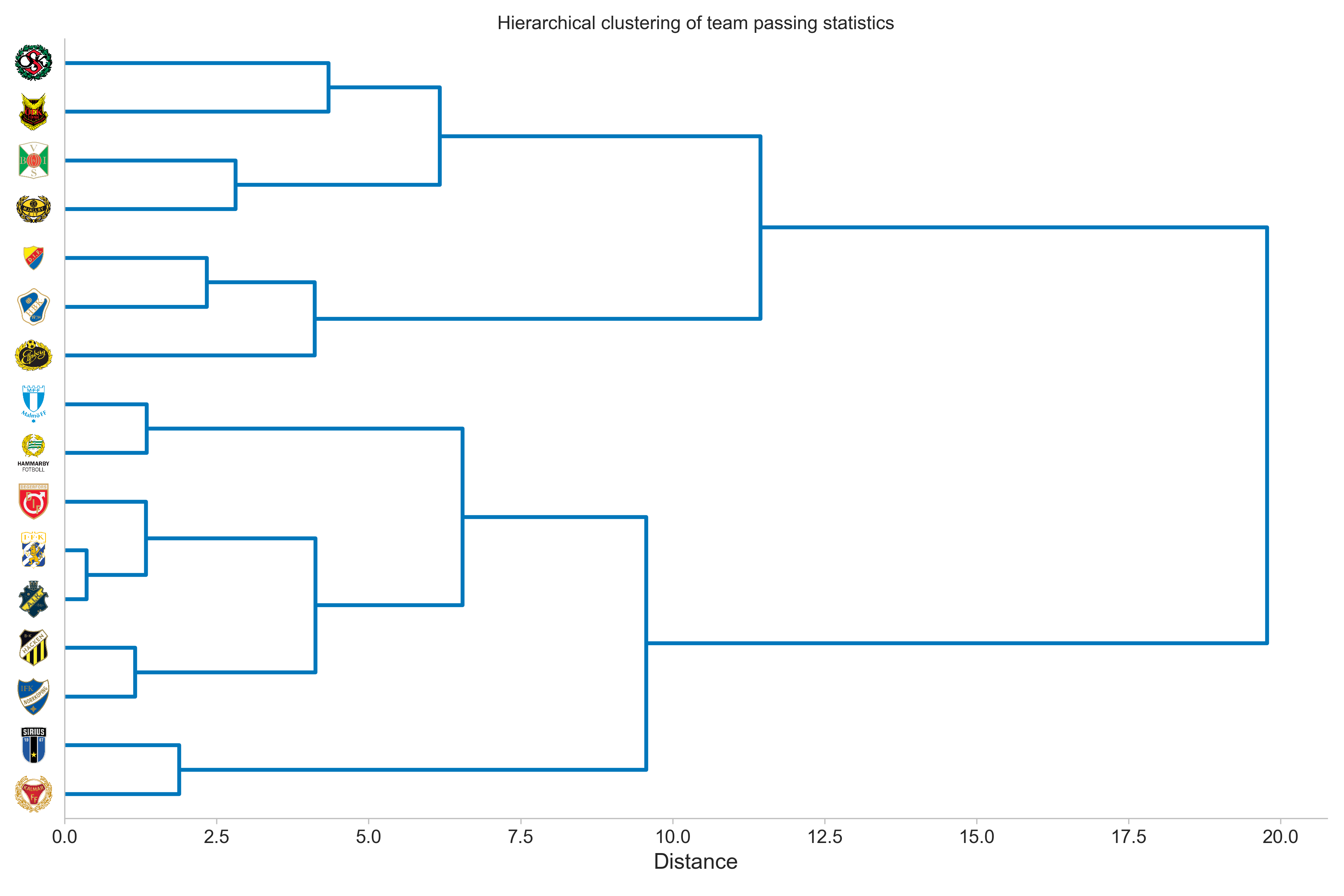
Here we can see that some of the observations from the scatter plot ring true. Namely, the teams inclined to short passing are in the lower half of the tree, while long passing teams make up the top half. Additionally, the two bottom teams (Örebro and Östersund) seem to be similar, which is also true for AIK and IFK Göteborg, the latter being the two most similar teams.
Now what we have a tree, i.e., clustering, to examine we can perform an analysis. However, we can first see the step-wise procedure that is used to create the final clustering you saw above.
An additional benefit of seeing it in this iterative way is that we can get a feel for where we can cut the tree. We want to cut the tree at a given point to form clusters, rather than the root cluster that contains all teams in one cluster. For instance, let us consider a cut-off distance of five. That is, we create clusters based on where they are when the distance is five units, which is indicated by the vertical gray line in the plot below.
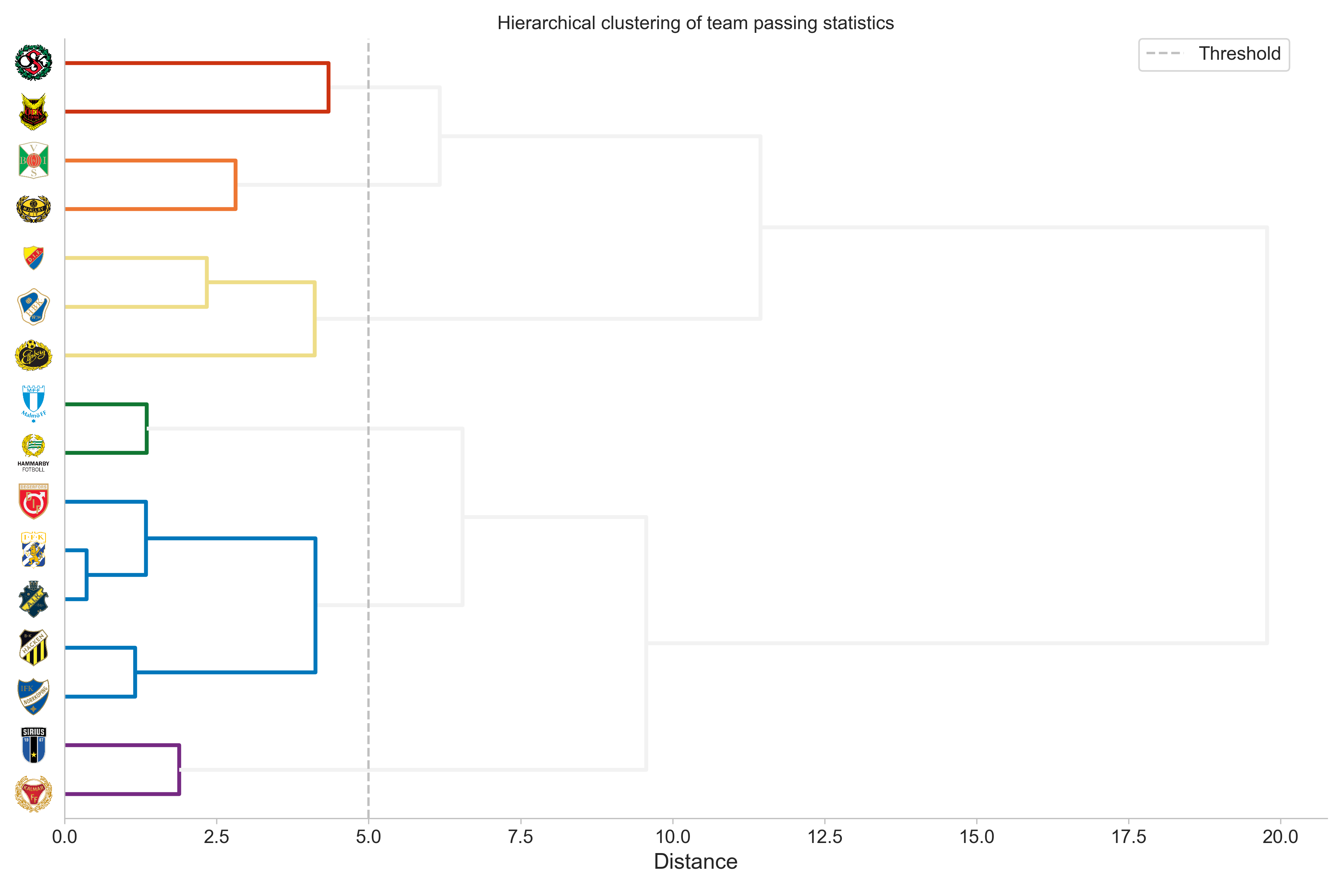
From this, we have six clusters in total, each given a unique color. The gray color indicate an unused link. With these clusters obtained, we can also investigate how the passing varies between (and within) clusters.
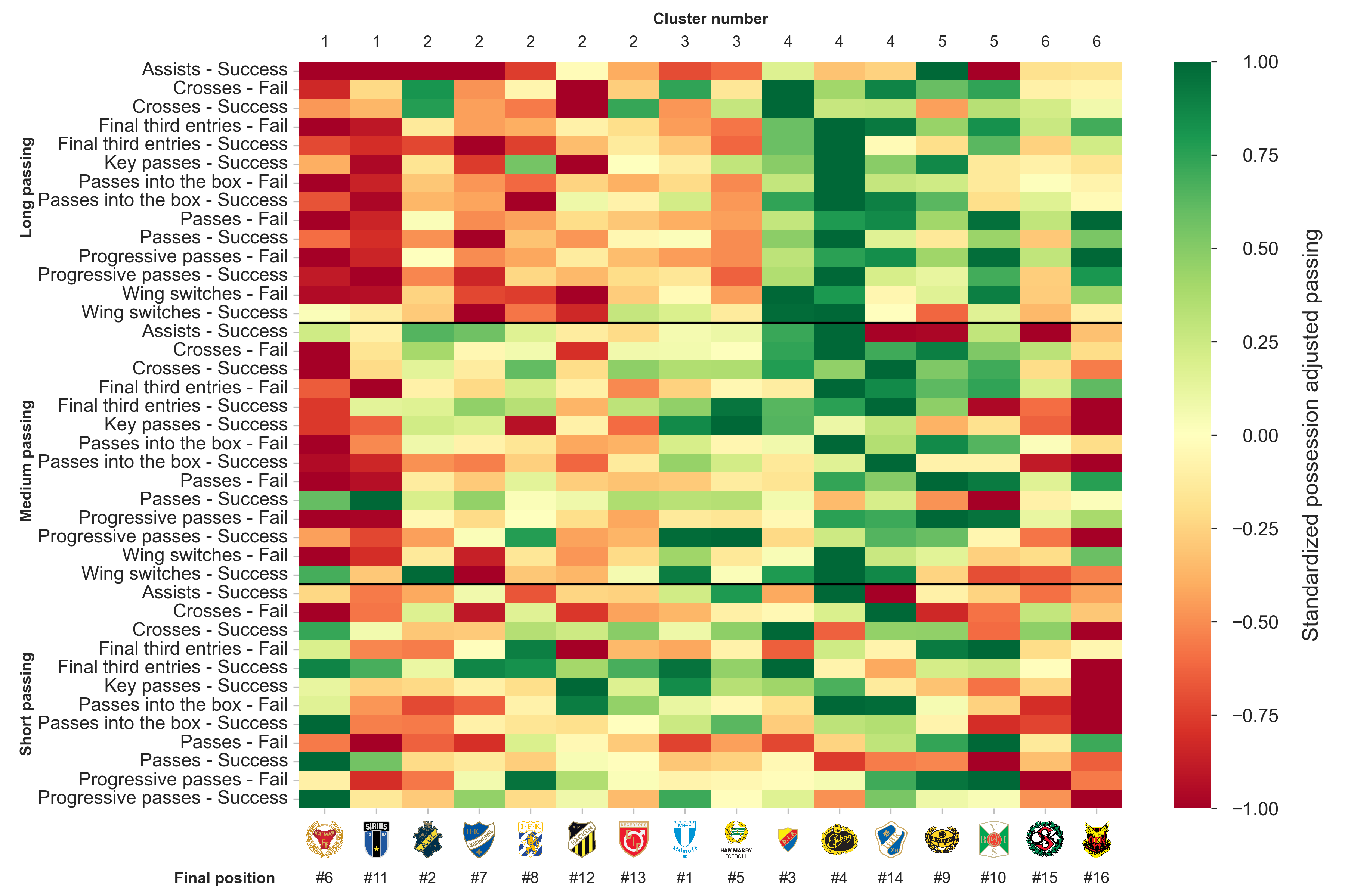
An initial observation that stands out is the distinction between short and long passing teams, evenly divided into three clusters each.
Short passing clusters
The short passing clusters (1, 2, and 3) in general do not play very much long passing, although some exceptions exists, e.g., AIK and their long crossing. Instead, Kalmar and Sirius both prefer to play it short with a lot of successful short and medium passes, but unfortunately they do not make this possession count in the way they would want, as the assists, key passes and passes into the box are only league average. On the contrary, Malmö and Hammarby that make up cluster 3, do just that: creating goal scoring opportunities by getting the ball into the box and into dangerous areas near the opposing team’s goal. They also tend to move the ball forward a lot, another indication of their offensive tendencies and attacking intentions. The last short passing cluster, which consists of AIK, IFK Norrköping, IFK Göteborg, Häcken and Degerfors, has more of a mixed bag when it comes to passing. AIK ranks highly in long crosses and mid-range wing switches, while IFK Norrköping and IFK Göteborg attempt many short final third entries, Häcken have many short key passes and failed passes into the box, and Degerfors do not stand out in any particular category.
Long passing clusters
The remaining three clusters (4, 5, and 6) have a tendency toward long passing and contains mainly lower ranked teams. However, there are two exceptions: Djurgården and Elfsborg. So what sets them apart from the other long passing teams? Well, the key things are that these two teams pass the ball forward into more dangerous positions, which can be seen by the highest number of passes into the final third, the box, and key passes. Curiously though, is that they are grouped together with Halmstad, who finished 14th and ended up being relegated. Why is that? Although it is not shown in this analysis, as the focus lies elsewhere, a major reason is the difference between expected goals (xG) and actual goals scored. According to their total xG4 Halmstad were expected to score between 35 and 36 goals, but only managed to score 21. With respect to passing however, they played similar to Elfsborg and Djurgården. Among the remaining four teams, the main difference is that the cluster with the bottom two teams, Örebro and Östersund, were quite reliant on playing long balls and hoping for the best, as they ranked near the bottom for all short passing categories. The final cluster is inhabited by Mjällby and Varberg, which, unfortunately for them, ranked highest when it comes to failed passing attempts. These failed passes are not only long passes as it also applies for short and medium distance passing.
A note on cluster quality: When it comes to any type of statistical analysis, it is always desirable to obtain r and metricsesults that are of the highest possible quality. When it comes to clustering, many different methods exist for evaluating the cluster quality and they all give some insight into how well the algorithm worked. For HAC, one such metric is the cophenetic distance/correlation coefficient, which (simplified) compares the pairwise distance of the (original) observations and the clusters produced by the algorithm. This metric ranges from -1 to 1, with values closer to 1 indicating that the clustering the original pairwise distances are preserved. In this case, the cophenetic coefficient is approximately 0.67, which can be seen as somewhat low but overall, I would still say the clustering provides some insights of value. And it is not common for clustering to produce perfect results in practice, as there is (almost) always some noise and/or unexplained variation in the data that may not be captured.
Future considerations: To conclude, I would like to add some closing remarks. Firstly, the data used for this analysis captures a lot of information regarding passing, but it does not capture all of it. For instance, consider the difference between a long pass from goalkeeper to central midfielder and a pass from a central midfielder over the defensive line. One of these is (typically) more dangerous than the other but that information is not captured, as we do not have access to where the other players are located. Information regarding pressure could also give additional nuances to the analysis, as it is reasonable to expect that some teams play more passes when pressured and the success rate also varies. In general, by combining this event data with tracking data, we could find even more insights, which will hopefully be possible in the future.
Acknowledgements
I would again like to thank PlaymakerAI for making their data available, and I will also extend my gratitude to the reader of this post!
References
[1] Tom Decroos et al. “Actions Speak Louder Than Goals: Valuing Player Actions in Soccer.” In: Proceedings of the 25th ACM SIGKDD International Conference on Knowledge Discovery & Data Mining. 2019, pp. 1851–1861.
-
It is worth noting here that since the number of variables outnumber the number of observations ($p=40$ > $n=16$), we can at most obtain ($\min(40, 16)-1$ = $16-1$ = $15$) principal components. ↩
-
Hierarchical clustering scales poorly with increasing sample size, as the general time complexity for obtaining a solution is typically $O(n^3)$. ↩
-
For more technical information, the reader is referred to e.g. Wikipedia or the original paper. ↩
-
Also computed from the data provided by Playmaker. ↩