Passing styles in Allsvenskan 2021

Have you ever thought about the most common event in football, the pass, and the various ways it is possible to play it? Well, look no further! In this post, we conduct an unsupervised learning clustering approach to detect the various passing styles prevalent in Allsvenskan during the 2021 season.

Introduction

No action is as prevalent in the game of football as the pass, whether it be a short pass between center-backs or an attempt at a crucial through ball to send the striker through on goal. It has been found that approximately 65% of all actions are passes [1]. As it is by far the most common action in football, passes represent a crucial component of a player’s playing style. Consequently, it is likely that not all players share the same passing style, but which passing styles and how many styles are there actually? Continue reading to find out!

For the code of this analysis, refer to this Github repo.

Data

The data originates from the open data repository of PlaymakerAI and without it, the rest of this work would not be possible.

As for the data used for the analysis, it contains all games in Allsvenskan during the 2021 season. Each game consists of approximately 1200-1500 actions that describe the events that take place during a game, e.g., passes, shots, tackles etc. Furthermore, each action is also described by what (the action taking place), who (the player and team performing the action), where (start and end $x$ and $y$ coordinates), and when (start and end time).

Pitch plot

To give a feeling of where the actions take place, refer to the following figure:

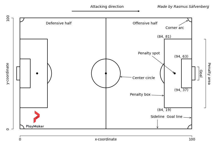
where each team always attacks left to right.

Selecting passing variables

From the data, the first step was to determine which passing variables could be derived and analyzed. The following variables were included:

Variable	Description	Length	Outcome
Assist	Pass leading to goal.	Long/Medium/Short	Success
Cross	Pass from the wing to the central attacking third.	Long/Medium/Short	Success/Fail
Final third entry	Pass from outside that enters the final third.	Long/Medium/Short	Success/Fail
Key pass	Pass leading to a shot or goal scoring opportunity.	Long/Medium/Short	Success
Pass into the box	A pass that ends inside the penalty box.	Long/Medium/Short	Success/Fail
Pass	All passes, with the exception of goal kicks.	Long/Medium/Short	Success/Fail
Progressive pass	According to the Wyscout definition.	Long/Medium/Short	Success/Fail
Wing switch	A pass going from wing to wing, at least half the pitch width.	Long/Medium	Success/Fail

Variables regarding corners and clearances were excluded due to the corners not being in open play and clearances not always being a pass, as well as lacking end coordinates.

Exploring passing variables

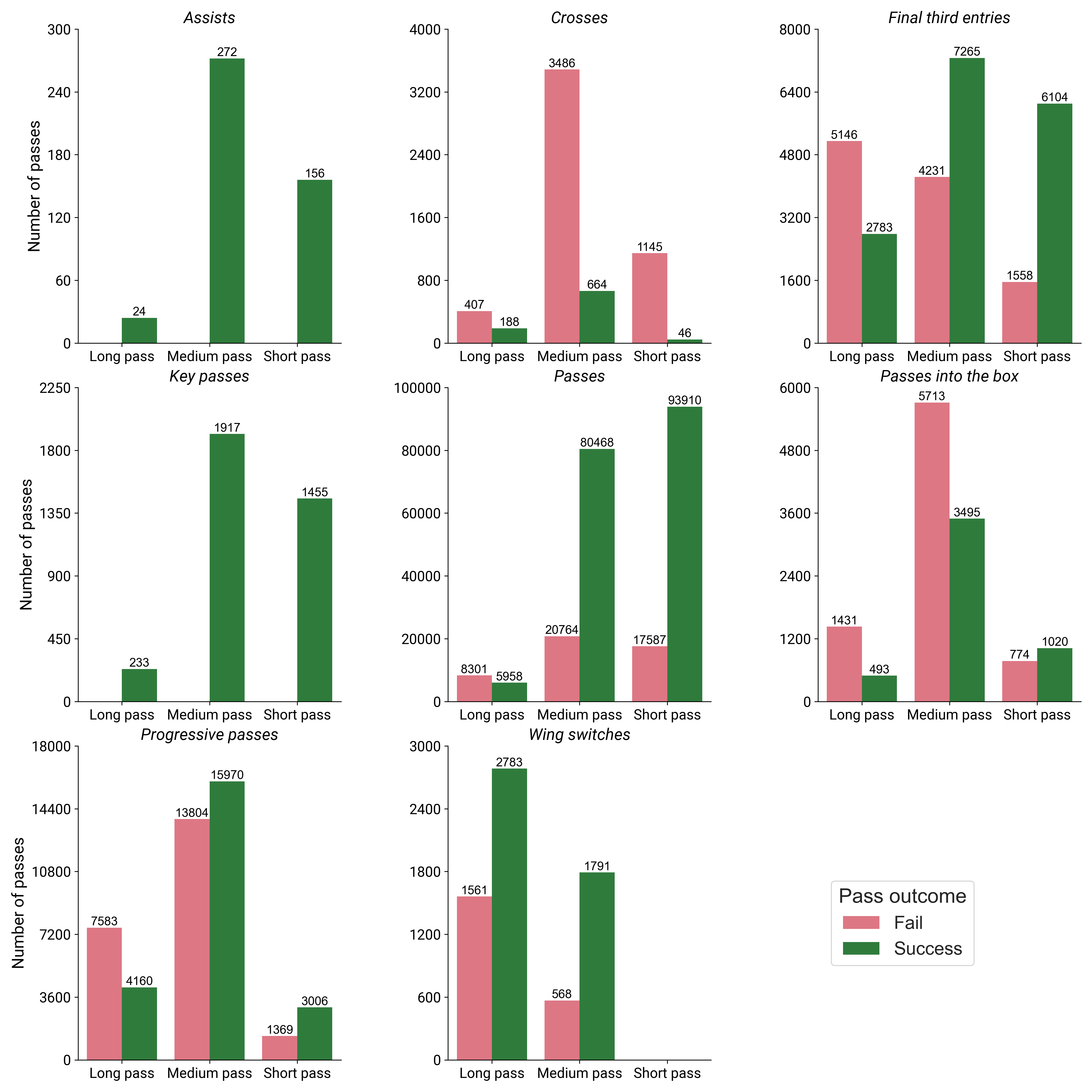
Prior to the analysis, we can as a first step investigate the number of passes per category as well as their rate of success. The counts given are total for all teams and games across the entire season. Also note the fact that they y-axes are different for each plot.

Preprocessing

After retrieving the data the next step is to process it such that an analysis can be performed. In particular, the data should be transformed from long to wide.

Data in long format is characterized by multiple rows describing the same action, e.g., a pass that is also a cross would therefore span two rows, one for the pass and another for the cross. However, for the analysis that will follow, the data should be in wide format, where each row describes a unique action. In the wide representation, each action will therefore be represented by the most succinct action, where in the previous example the pass would be be described as a cross (as a cross is also a pass, but the opposite need not be true).

Although, this is the general procedure, some actions are not kept in the same way. These actions are assists, key passes, and passes into the box. This is due tothe basis for the analysis being founded on the SPADL definition from [1].

Further preprocessing steps include:

1. Create a separate column containing the result of each action (success/fail).
2. Adding boolean columns for key passes, assists, and passed into the box to indicate whether the pass also has one of the additional tags.
3. Transforming the pitch coordinates to $x \in [0, 105]$ and $y \in [0, 68]$.
4. Computing the distance of passes.
5. Determining if a pass was a progressive pass or not.
6. Adding a column for the passing length, which is defined as:
   • short, if the pass distance is less than 15 meters, or
   • medium, if the pass distance is between 15 and 40 meters, or
   • long, if the pass distance exceeds 40 meters.
7. Computing the number of passes per result and pass length for each player in each game.
   • Note that goal kicks and goalkeeper throws are excluded in this step.
   • The player's value is then divided by the minutes played in the game.
   • And in turn, the value is then also divided by the possession his team had in the game.
   • Next, the value is multiplied by 90 to represent the count per 90 minutes.
   • In this step we also filter out players who played less than 300 minutes during the season.
8. After computing these standardized statistics, the next step is sum the to be for the entire season.
9. Finally, before feeding the data to the next step, we normalize the data by subtracting the mean and scale to unit variance. This ensures the variables are all on the same scale.

Whew! That was a “short” summary of the preprocessing! If you would like to check the preprocessing in detail, check out the scripts in the Github repo.

Method

How should we go about finding these different passing styles? Well, there are various ways this analysis can be done. However, the most common way to group observations (in this context, players) is through clustering as it can provide qualitative groupings without the use of an explicit label.

Unsupervised learning

This analysis is founded on unsupervised learning, which is a machine learning algorithm to learn patterns from data without using a target/label. Common machine learning algorithms aim to solve problems regarding, e.g., dimensonality reduction and clustering.

Dimensionality reduction

Prior to performing the clustering, it is worth noting that the distance between two points in a high-dimensional space is typically not as well-behaved as one would like. As a result, the distance may contradict our intuition and what we believe makes sense. One way to alleviate these possible issues is to reduce the dimensionality of the data. A popular method for this is principal component analysis (PCA), where all the original variables undergo a transformation.

More specifically, in PCA, a linear combination (called components) of the original variables is created such that each variable contributes, positively or negatively, to some extent, some more than others. Each component is orthogonal to the previous and strives to maximize the variance in the data, which means that the first component has the highest variance explained in the data, followed by the second component and so on. The aim with this is to represent as much of the information as possible in a lower dimension.

For instance, if the original variables are 100 in total, with PCA this may be able expressed at a satisfactory level with only a few components, say 2-5. This can then improve the result of the clustering that follows and can also allow visualizations in a lower dimensional space.

One thing that is also worth mentioning is that PCA, in its original form, always return the same number of components as original variables and to reduce the dimension a choice has to be made of how many components should be retained. Many methods exist to accomplish this and the author’s choice is to use parallel analysis [2]. This method is outside the scope of this text, but it generally performs better than selecting the number of components manually, by e.g., selecting a minimal threshold of variance explained.

Clustering

In the next step, after performing PCA and obtaining a set amount of components, we can finally move on to the fun part, clustering! The method of clustering revolves around grouping objects into a set of groups, that are called clusters. Many algorithms also exist for this purpose, and the choice here is that of partitioning around medoids (PAM) [3], which is a solution to the $k$-medoids problem.

In short, PAM searches for $k$ objects (here, players) to represent the center of each cluster. Each cluster center is referred to as a medoid, which is a also represented by one of the objects, as opposed to $k$-means. Each object is assigned to the cluster to which the object is least dissimilar, and in general it is less sensitive to outliers than $k$-means.

Similar to PCA, a choice also has to be made regarding the number of clusters. To do this, we can compare e.g., the silhouette score, which describes how distinct the clusters are. A higher value is better, although the choice need not always be the $k$ that gives the highest value.

Results

Let us now move on to the results.

PCA

Firstly, let us investigate the how much of the variance of the data each principal component explains.

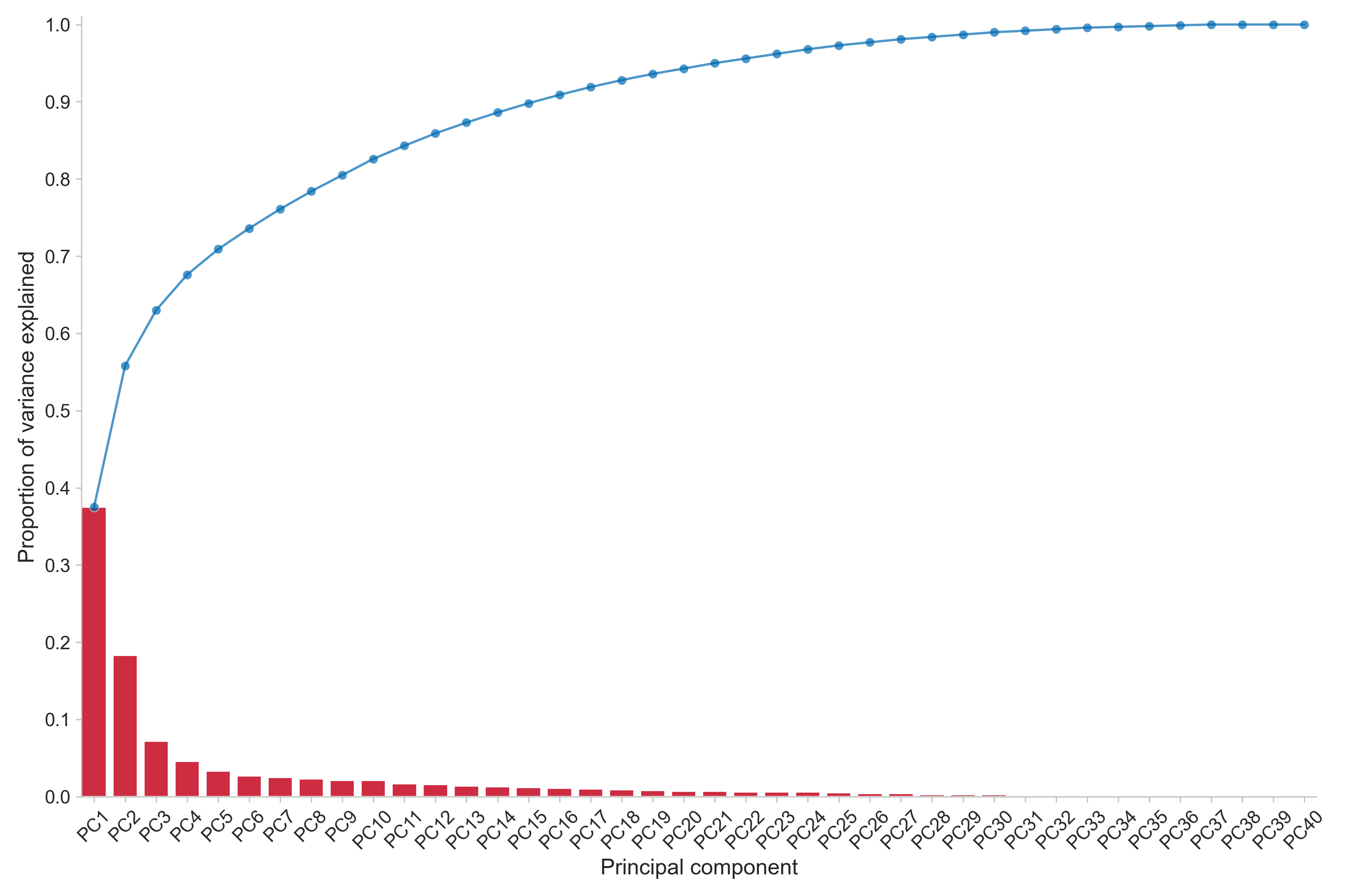
In the figure, where the red bars show individual component values and the blue line describe the cumulative proportion of variance explained, we can see that the first two components explain approximately 55% of the variance in the data. The first component alone is responsible for slightly below 40% of the total. If we extend this to the first four components, which is also how many components the parallel analysis suggest we retain, 70% of the variance is explained. Naturally, we would like to explain all of the variance, but this is rarely the case in practice as the data may have sources of variation that are difficult to compress.

Next, we can examine the PCA loadings. That is, how much each variable contributes to each principal component. The loading ranges from -1 to 1, where a larger absolute value describe that a variable has stronger influence on the component.

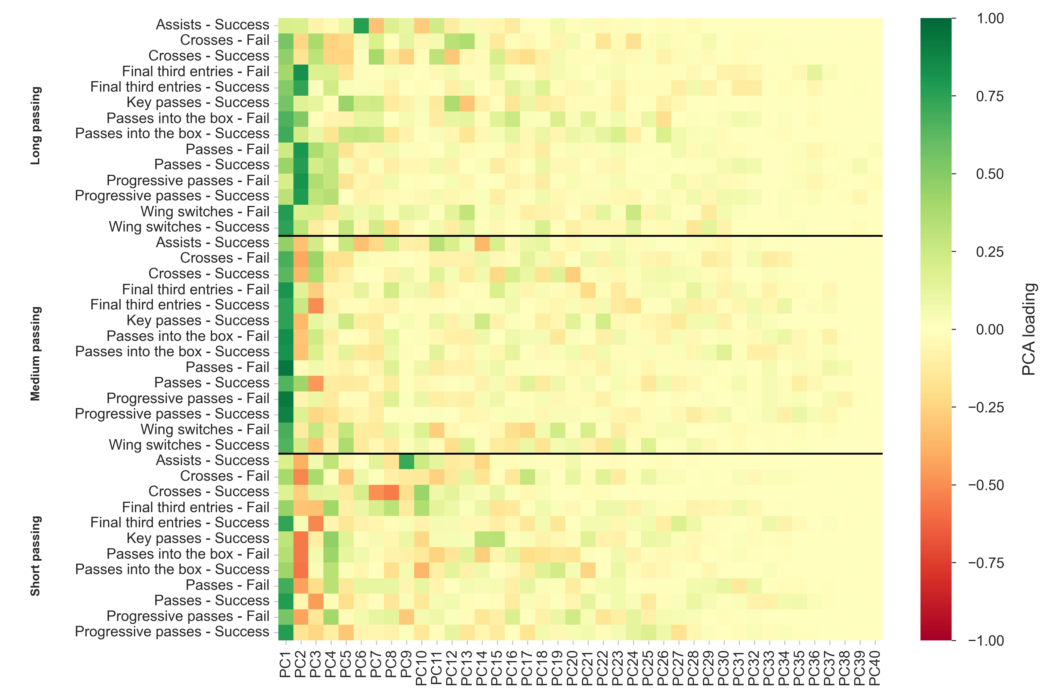
As the figure shows, nearly all of the variables have a positive influence on the first component, although some are near zero. Meanwhile, the second component is mostly influenced by long passing (positively) and short passes into the box (negatively). Furthermore, short and medium passes impact the third component while short key passes and passes into the box are most influential for the fourth component. The later components are in general typically not heavily influenced by many variables and tend to be close to zero.

Clustering

After the dimensionality reduction, we proceed to clustering. But first, a decision has to be made on how many clusters to use. For this, we examine the silhouette score to measure the optimal number of clusters, with respect to distinct clusters.

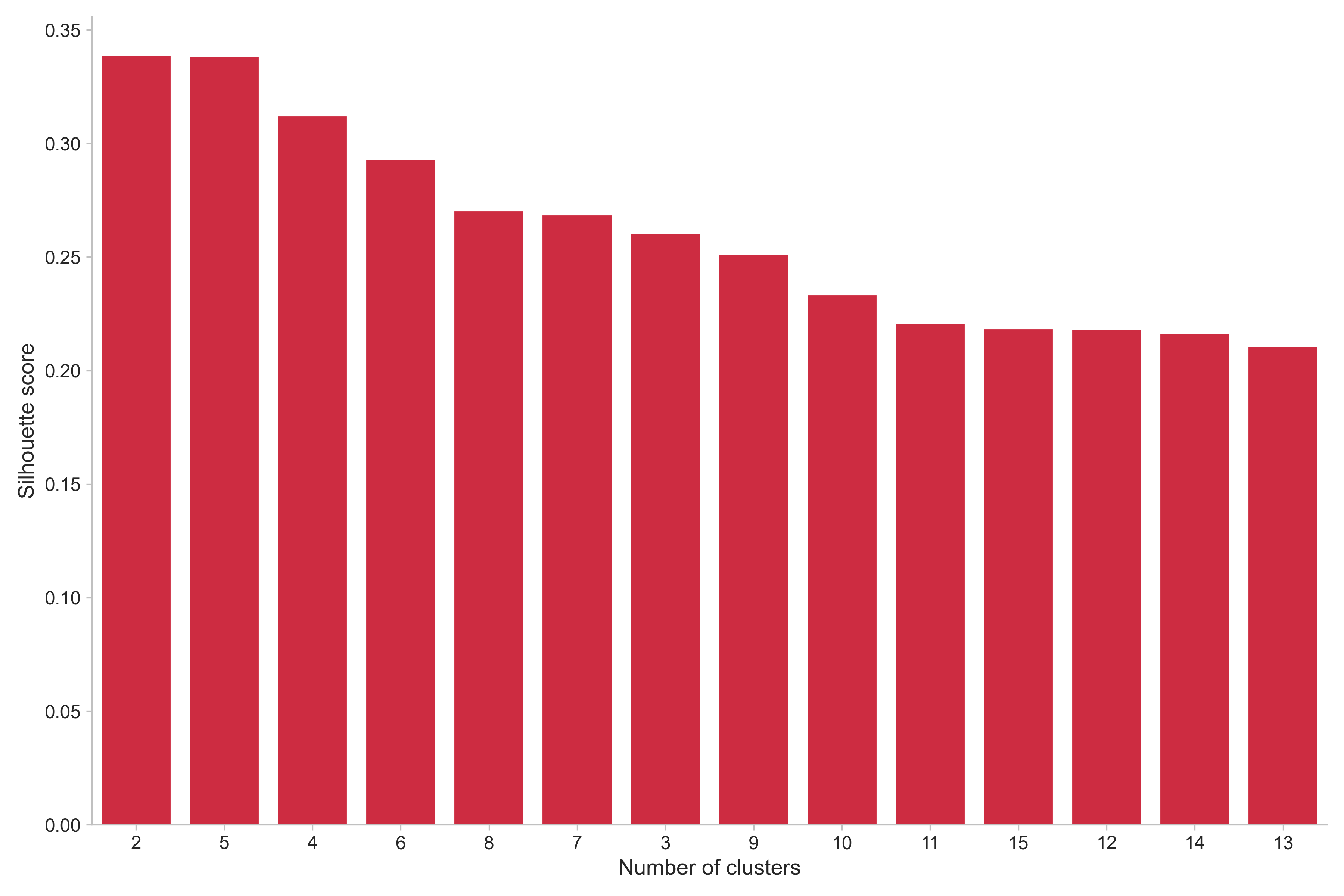
Based on this, the five choices that are deemed most distinct are 2, 5, 4, 6, 8. However, it can be argued for the purpose of this investigation that 2 clusters will not provide a satisfactory level of distinction between different players. After examination, neither 4 or 5 clusters achieved this. Therefore, the choices are either 6 or 8 clusters. To choose between them, both were investigated (visually and qualitatively) and, from domain knowledge, having 6 clusters was missing a distinction between players that disagreed more with intuition than 8 clusters. Thus, 8 clusters were chosen.

Once the number of clusters had been determined, a thorough evaluation of the clusters could be performed. For a fast overview, let us examine the means and rankings of each cluster among the variables.

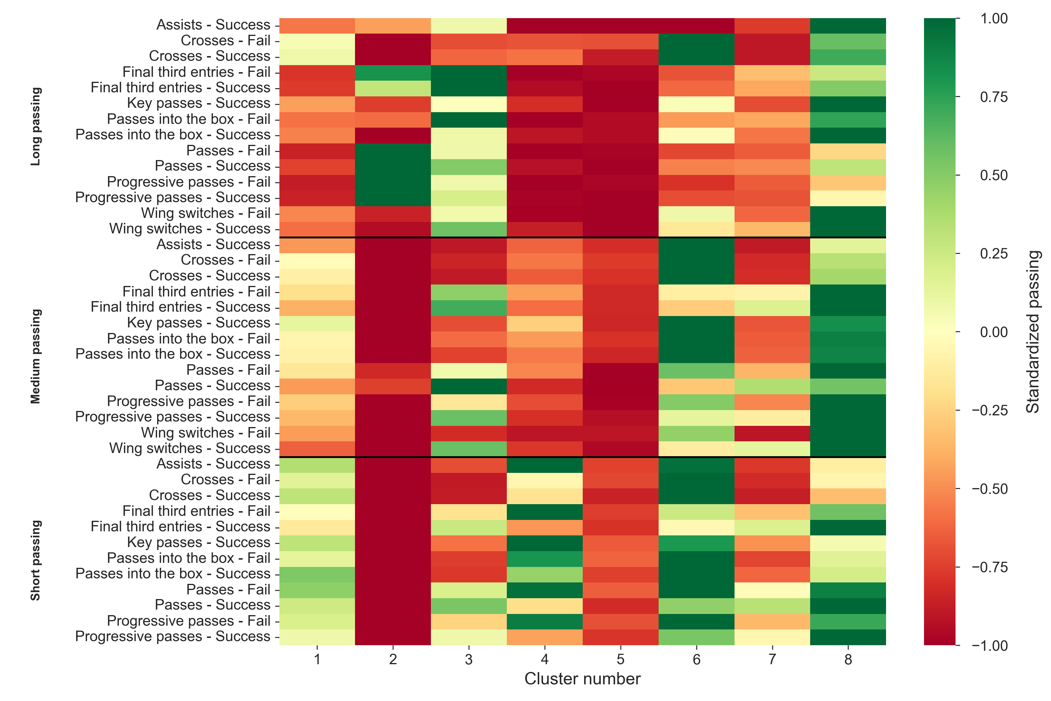
The first thing to note is that cluster 8 is the cluster where the highest ranking players reside, which means they are the players who are the most notable passers. On the contrary, cluster 2 and 5 ranks low in most categories, except in the long passing categories for cluster 4. Similarly, cluster 3 also ranks highly in long passing, but also in medium distance passing and wing switches. Meanwhile, cluster 1 and 6 rank highly in crossing and key passing, where cluster 6 tends to rank higher. Finally, cluster 7 ranks near average across all categories.

Positions within each cluster

It is also worth exploring how the (primary) playing position, according to TransferMarkt¹, varies between cluster.

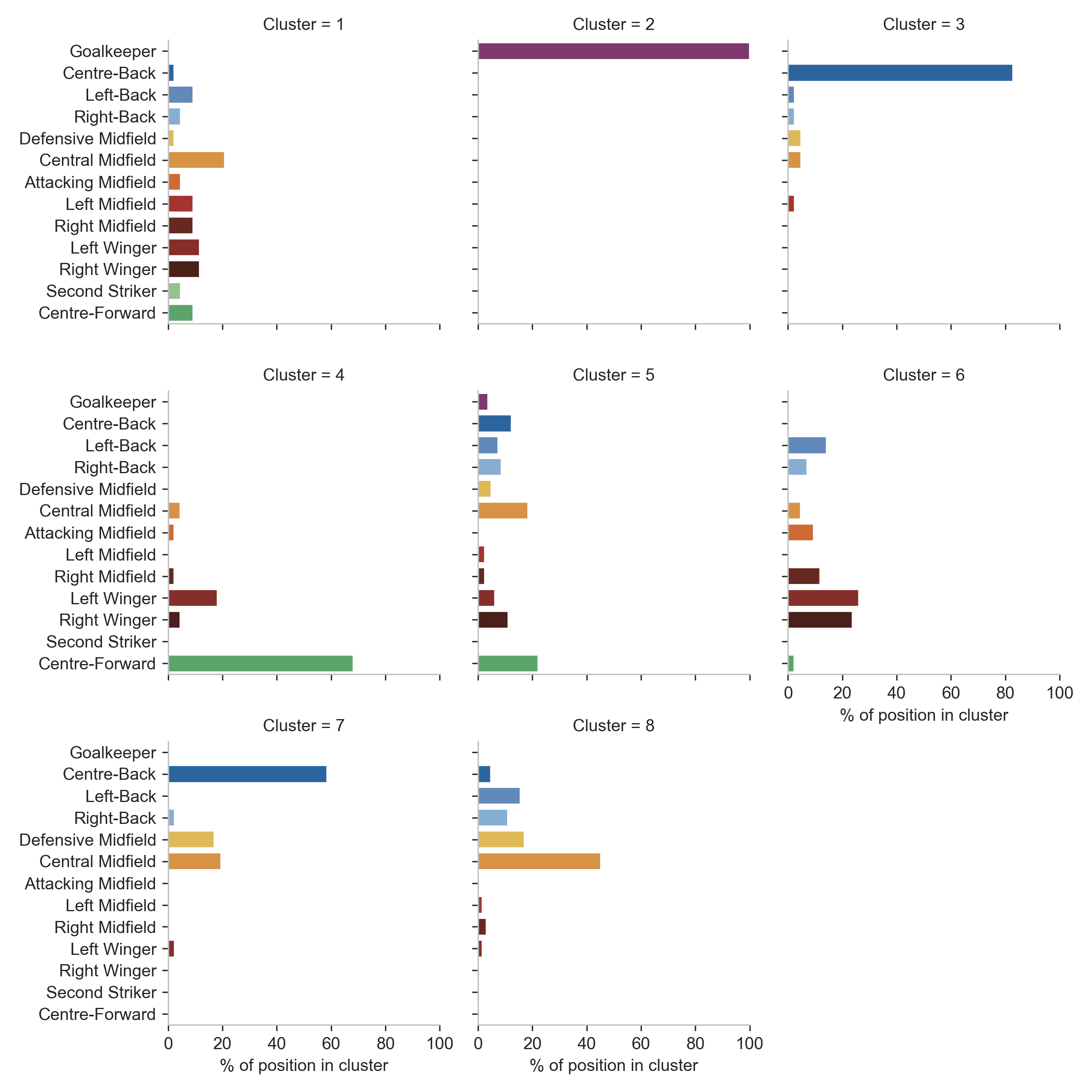
As the figure entails, cluster 1 and 5 have a rather varied set of players from many positions. On the other hand, cluster 2 (goalkeepers), cluster 3 and 7 (center-backs), and cluster 4 (forwards) are all dominated by one position. As for the other clusters, central midfielders are the most common position in cluster 8 while cluster 6 contains mostly wide midfielders and wingers.

Labeling the clusters

Based on the previous results, the following labels for each cluster can be suggested:

Cluster	Label	Specialities	Rarities	Medoid2
1	The final third creator	Play in the final third	Long passing	Emil Tot Wikström (Halmstads BK)
2	The goalkeeper	Long passing	Everything else	Kristoffer Nordfeldt (AIK)
3	The defensive outlet	Medium and long passing	Crossing	Tobias Carlsson (BK Häcken)
4	The target man	Short key passes/assists	Long passing	Henok Goitom (AIK)
5	The unwilling passer	Nothing	Everything	Stefan Silva (AIK)
6	The winger	Crossing and passes into the box	Long passing	Patrik Wålemark (BK Häcken)
7	The defensive passer	Medium distance passing	Crossing, key passes/assists	Enoch Kofi Adu (Mjällby AIF)
8	The advanced playmaker	Everything	Nothing	Ísak Bergmann Jóhannesson (IFK Norrköping)

where specialities refer to types of passing the cluster performs more often and rarities are passing types that are seldom performed.

Passing style description

1. The final third creator: The style with the most variety in positions shares the common trait of cherishing play in the final third, although the player’s own passing entries into it are rare.
2. The goalkeeper: Self-explanatory. This style consists solely of goalkeepers whose specialties are long passing and typically rarely engage in the team’s passing network.
3. The defensive outlet: Here we will find mostly center-backs who excels in medium and long distance passing, while crossing is not their forte.
4. The target man: The target man is here describing the team’s primary penalty box presence, with a specialty for short key passes and assists (mostly within the penalty box). Their weakness is long distance passing.
5. The unwilling passer: The players who, during their time on the pitch, rarely attempt many passes and instead rely on other events to make their mark.
6. The winger: A wizard on the wings, the winger delivers crossing and wide play at a high rate, with many passes having a destination within the opposition’s penalty box. However, long distance passing is less common.
7. The defensive passer: Among the defensive passers we can a mix of central players from the defense and midfield that commonly plays safer passing, with a higher success rate. Their offensive contribution is rather limited though.
8. The advanced playmaker: The maestro that is essential in establishing and creation in the team’s attack, with by far the most passes made across a majority of categories.

Reminder: All passing statistics are possession-adjusted.

Visualizing the clustering

Another benefit of the dimensionality reduction performed by PCA is that we can also visualize the data in a lower dimensional space, e.g., two dimensions. Let’s do that!

As we can see, the goalkeepers can be found in the top left corner, the best playmakers in the middle right, the wide players near the bottom, and the unwilling passers below the goalkeepers.

For a more detailed exploration, refer to the interactive version:

Overall, the clustering highlight a grouping that aligns with one’s intuition. For instance, among the most prominent playmakers we find both Magnus Eriksson, who led the league in assists, and Johan Larsson, who was a prominent contributor for Elfsborg’s attacking prowess. Similarly, we can also find wingers, such as Mohanad Jeahze, Jonathan Levi, and Jonathan Ring, who frequently created danger from their wide positions. It is also natural that there exists a cluster for goalkeepers, although two goalkeepers were in another cluster.

Conclusion: To conclude, I would like to add some closing remarks. Firstly, the data used for this analysis captures a lot of information regarding passing, but it does not capture all of it. For instance, consider the difference between a long pass from goalkeeper to central midfielder and a pass from a central midfielder over the defensive line. One of these is (typically) more dangerous than the other but that information is not captured, as we do not have access to where the other players are located. Information regarding pressure could also give additional nuances to the analysis, as it is reasonable to expect that some teams play more passes when pressured and the success rate also varies. In general, by combining this event data with tracking data, we could find even more insights, which will hopefully be possible in the future. However, I would argue, based on the available information, that the resulting clustering captures what one might expect in regards to passing styles.

Acknowledgements

I would again like to thank PlaymakerAI for making their data available, and I will also extend my gratitude to the reader of this post!

References

[1] Tom Decroos et al. “Actions Speak Louder Than Goals: Valuing Player Actions in Soccer.” In: Proceedings of the 25th ACM SIGKDD International Conference on Knowledge Discovery & Data Mining. 2019, pp. 1851–1861.

[2] John L. Horn. “A rationale and test for the number of factors in factor analysis”. In: Psychometrika 30.2 (1965), pp. 179–185

[3] Leonard Kaufman and Peter J. Rousseeuw. “Partitioning Around Medoids (Program PAM)”. In: Finding Groups in Data: An Introduction to Clus- ter Analysis. John Wiley & Sons, Ltd, 1990. Chap. 2, pp. 68–125.

1. It is worth noting that TransferMarkt does not always have correct position labelling for all players. ↩

2. Medoid is just a fancy way of saying cluster center. ↩