Finding the most effective scorer in the NHL
As in many sports, the goal in ice hockey is to outscore your opponent. From your team’s perspective it would (of course) be preferable to score many goals on as few shots attempts as possible. However, we know in practice this is not feasible, as scoring on each shot you take will not happen. That being said, is it possible to find players who are the most effective when it comes to scoring? The code for this analysis can be found in this repo.
Shooting percentage
The metric of interest in this analysis is shooting percentage (S%), which is defined as the fraction of goals divided by the number of shots on goals. However, if we were to rank players as-is using S% then the best shooters (according to NHL.com/stats) in NHL history are:
| Player | Shots | Goals | S% |
|---|---|---|---|
| Garrett Pilon | 1 | 1 | 100 |
| Egor Korshkov | 1 | 1 | 100 |
| Matt Corey | 1 | 1 | 100 |
| Samuel Henley | 1 | 1 | 100 |
| Joe Whitney | 1 | 1 | 100 |
which, of course, is not depicting an entirely truthful picture as none of these players participated in more than 5 games. In total, there are 14 players who have a 100% shooting percentage but they have all only taken one shot each. However, we are not interested in these players as scoring on your first shot is not an accurate indicator of who is an effective scorer when accounting for volume (shot attempts). Instead, we will be using a shrinkage method known as empirical Bayes.
Data
For this analysis we will be using shooting data from all NHL players, scraped from NHL’s API, since the 1959-1960 season, as this was the first season where they tracked shots. The final season under consideration is the 2021-2022 season as this was the latest season with full season data. The data is reported at the season-level and consists of variables regarding the player, their handedness, position and team, the current season as well as number of shots and goals.
Exploratory data analysis
Before jumping into the modeling we should first examine what impacts shooting percentages. More specifically, we will investigate this for both single-season data as well as career data. As a starting point we may expect that there will be a difference between forwards and defenders, so let us examine that in more detail.
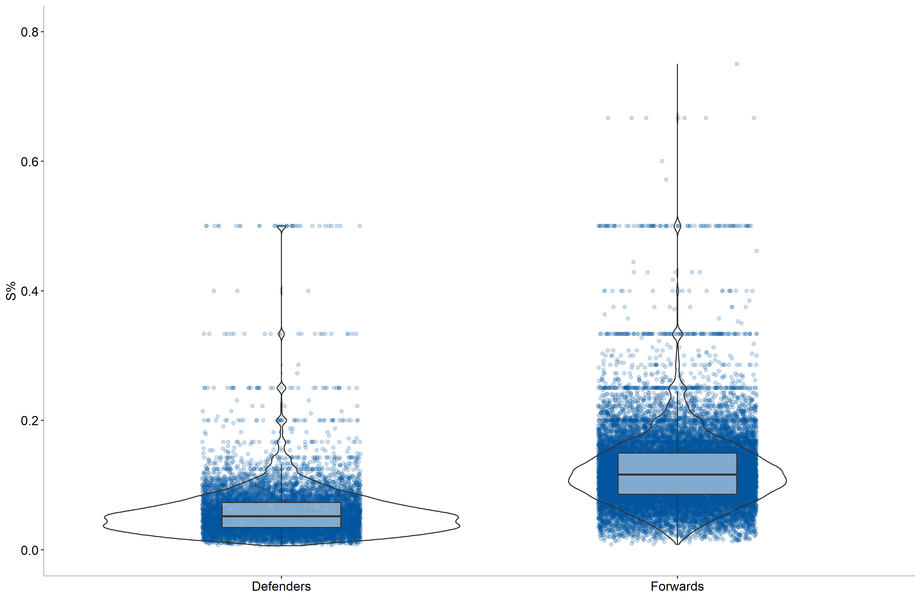
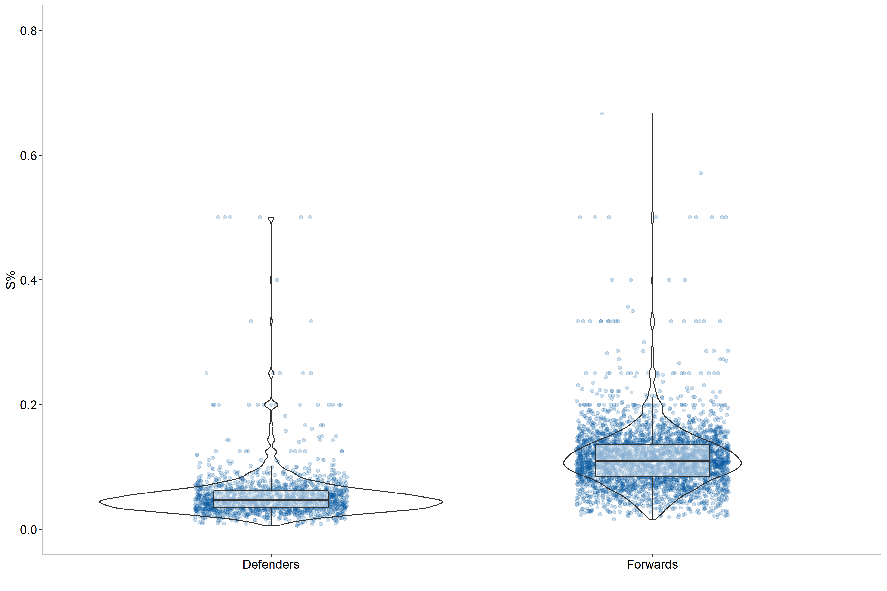
Here we can see that forwards tend to be more efficient shooters than defenders, which is logical as the offensive production is more emphasized for forwards. Moreover, defenders tend to shoot further from the net than forwards. We can also see some outliers, particularly for forwards, where some players have a 50% or higher scoring rate. This indicates that position should be included as a variable for our modeling, but we can do better. Let us also check if handedness matters, that is how the player shoots the puck.
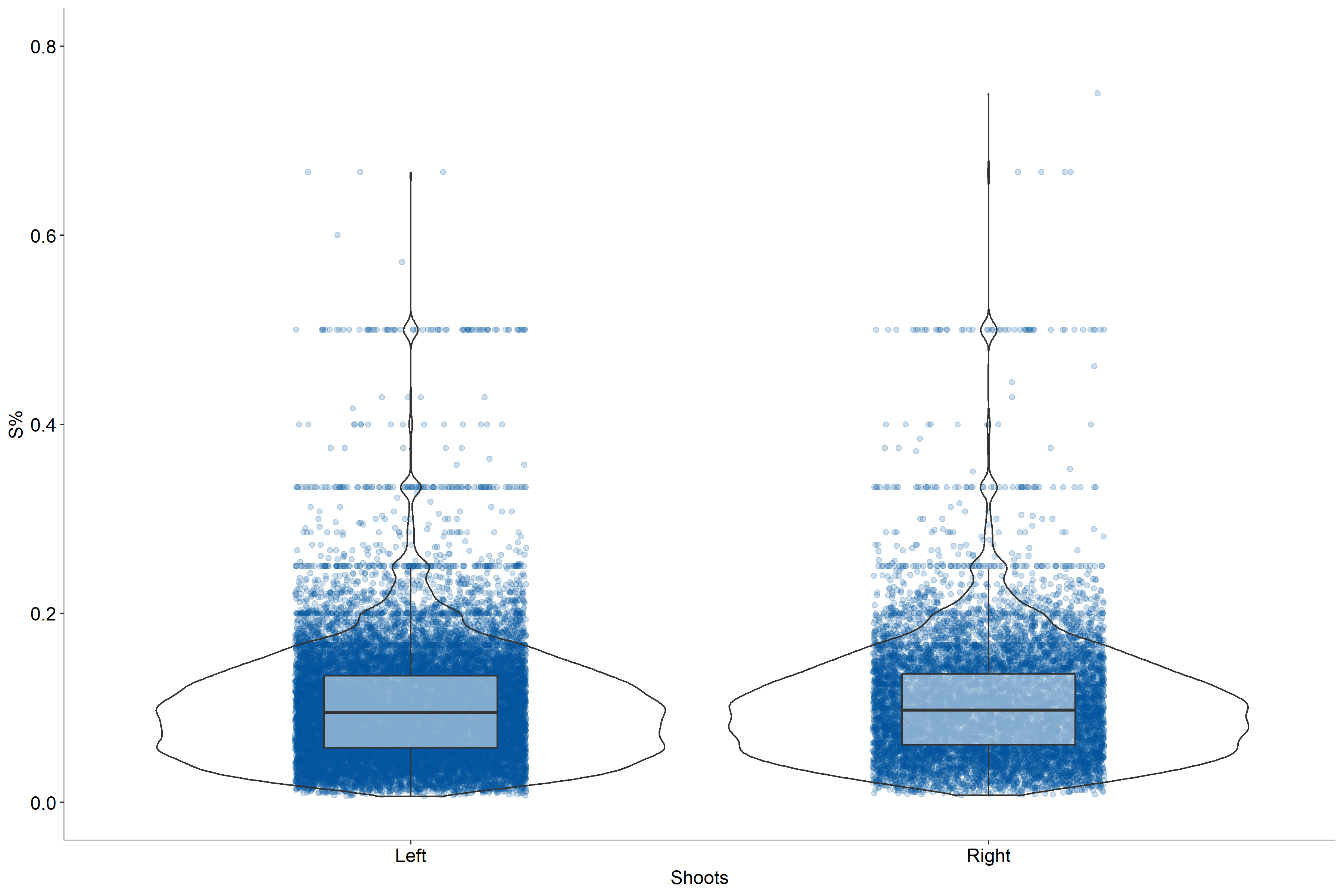
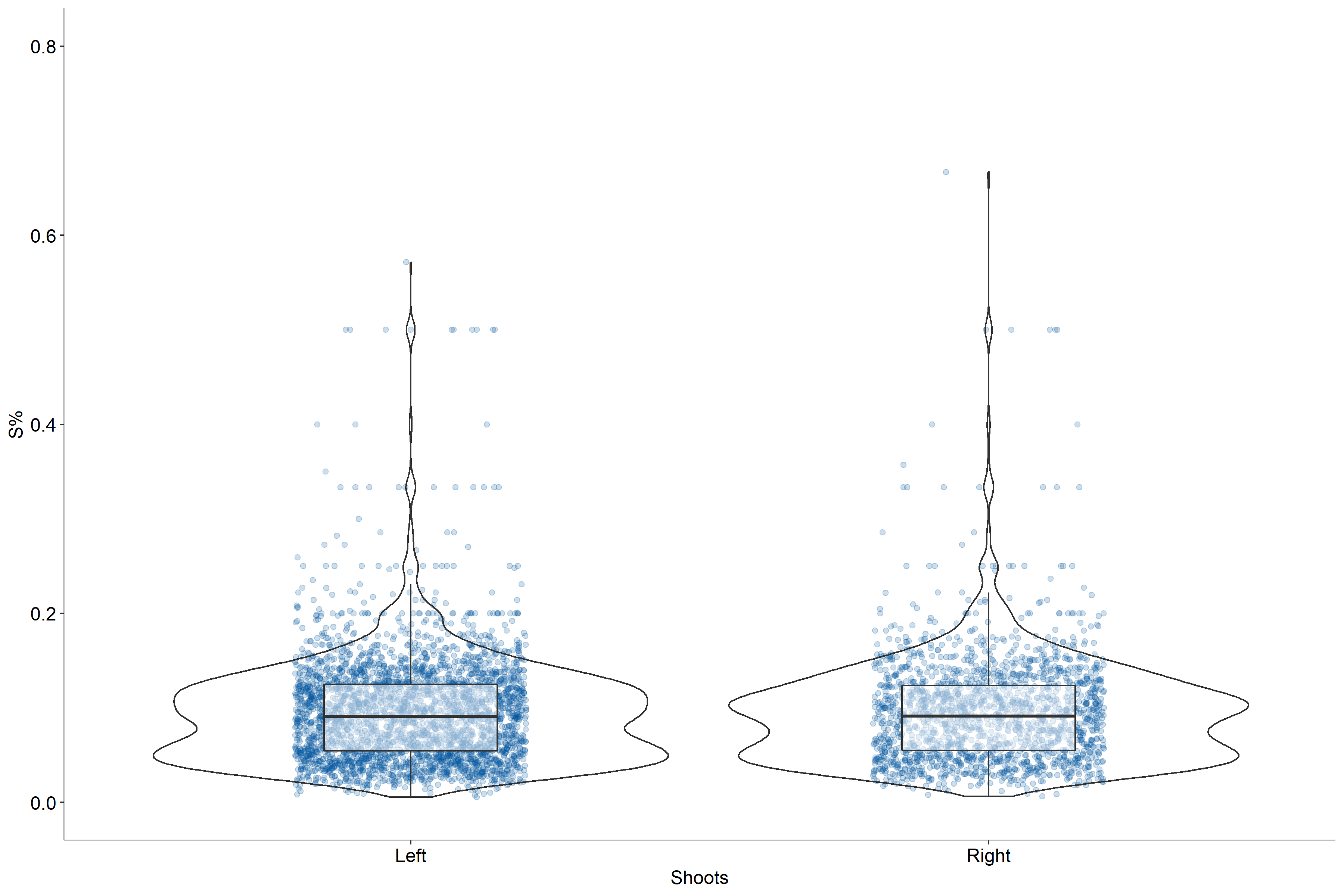
Based on this figure we can draw the conclusion that handedness does not seem to impact shooting percentages as the two distributions are near identical for both single-season and career numbers. As a result, we do not need to include this in our model.
Another aspect that we can explore is that of number of shots taken, as has been suggested in [2] as an improvement to [1]. In this case we may expect some differences in shooting percentages between players who took few shots and those who shot far more, which also applies for single-season values.
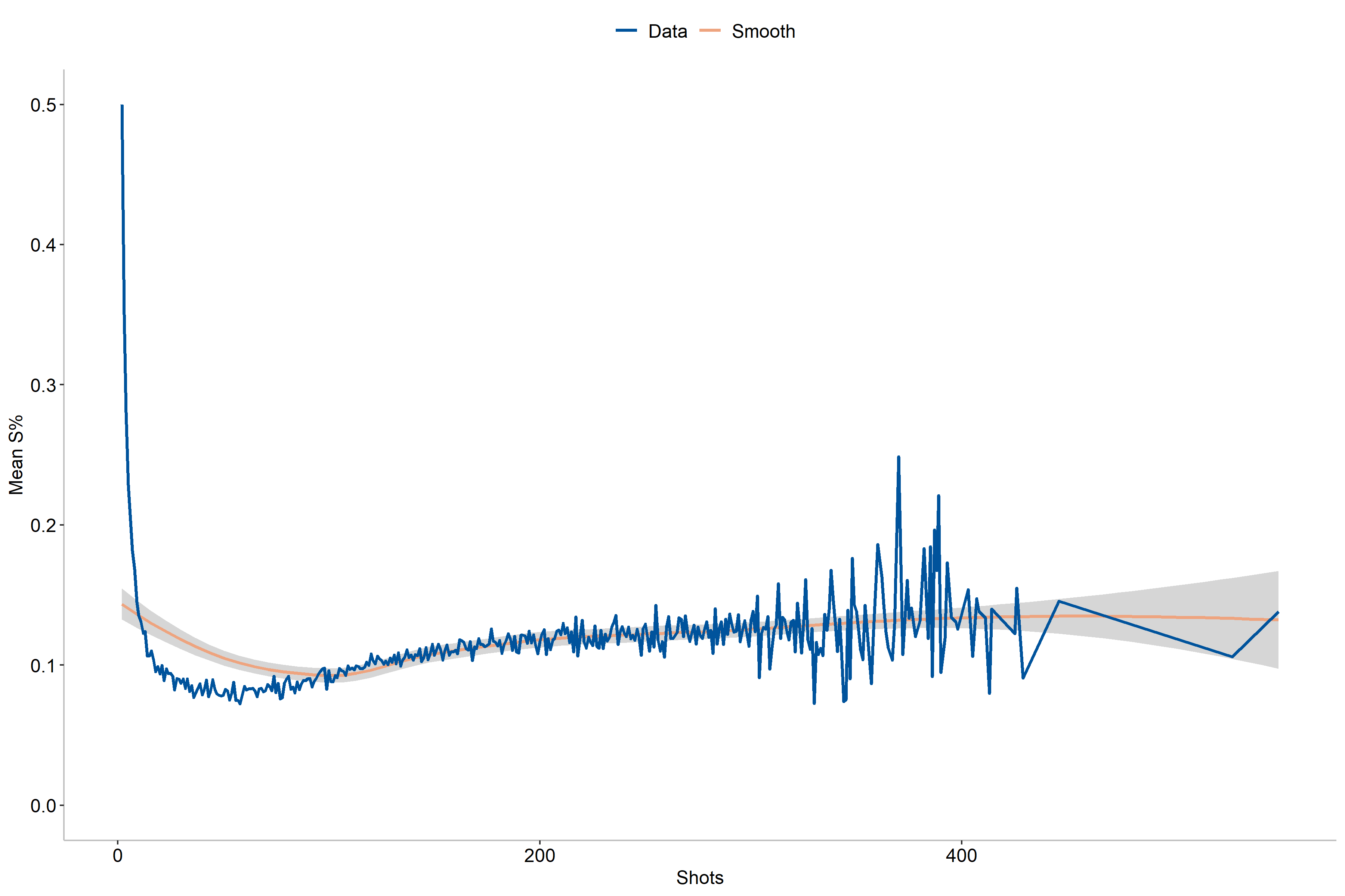
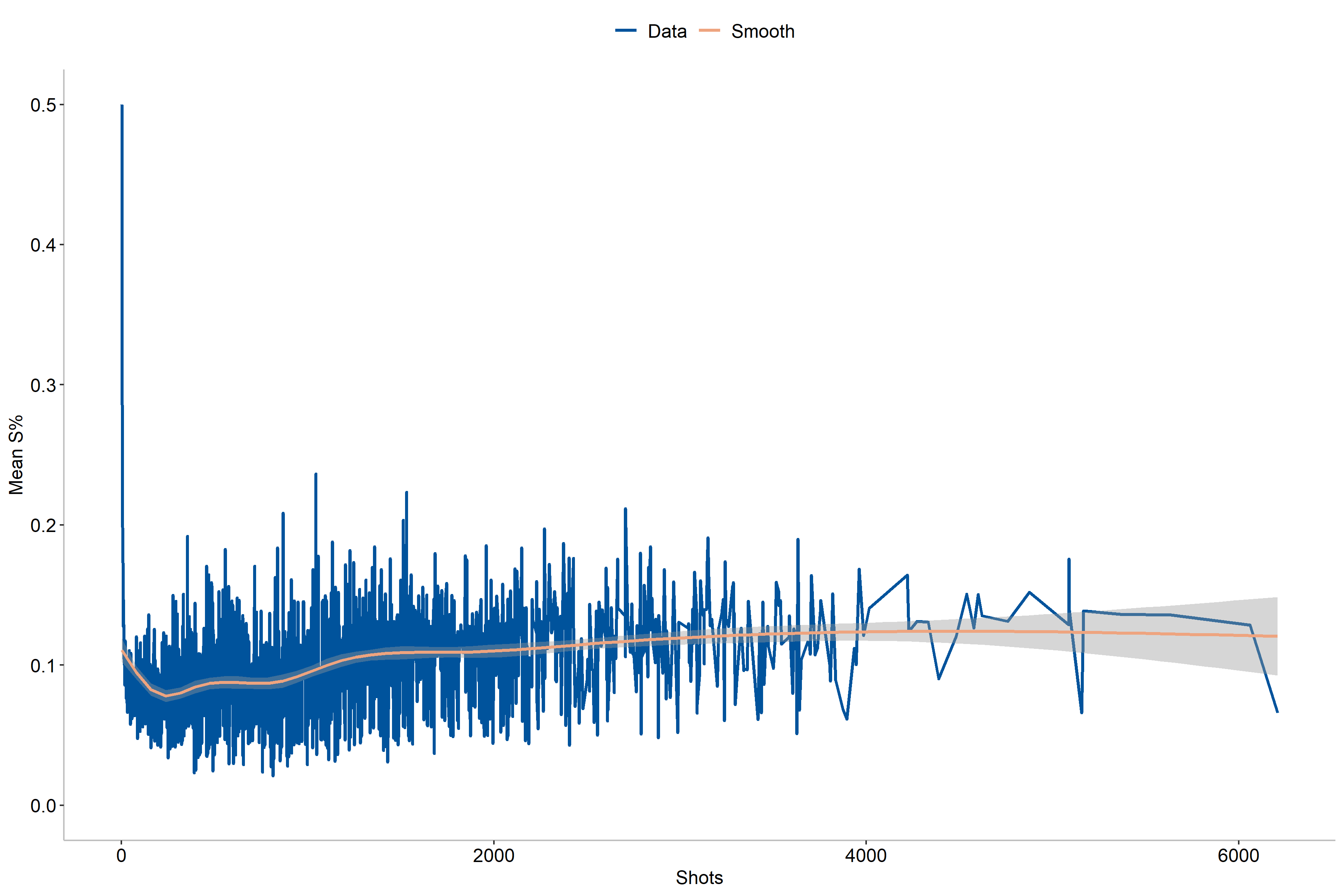
As the figures entail, we can see that the shooting percentages is the highest for players with the fewest shots taken, probably due to lower number of shots. Additionally, we see that the values tend to stabilize rather quickly with less variation when the number of shots increases. For single-season shooting numbers we also notice a slight increase in effectivity for the players who play a full season.
Finally, we may also reasonably expect that shooting has changed over time in the NHL. Our data covers data over a 60-year period and some change during this time is likely, so let us explore it. However, we should first note how years are treated for career numbers. Here I have chosen to compute the year for career numbers as the average year a player was active. For example, if a player had a 10-year career spanning from 1980-1990, the average will be 1985 and so on. The years correspond to the start year of a season, which means that 1985 correspond to the 1985-1986 season.
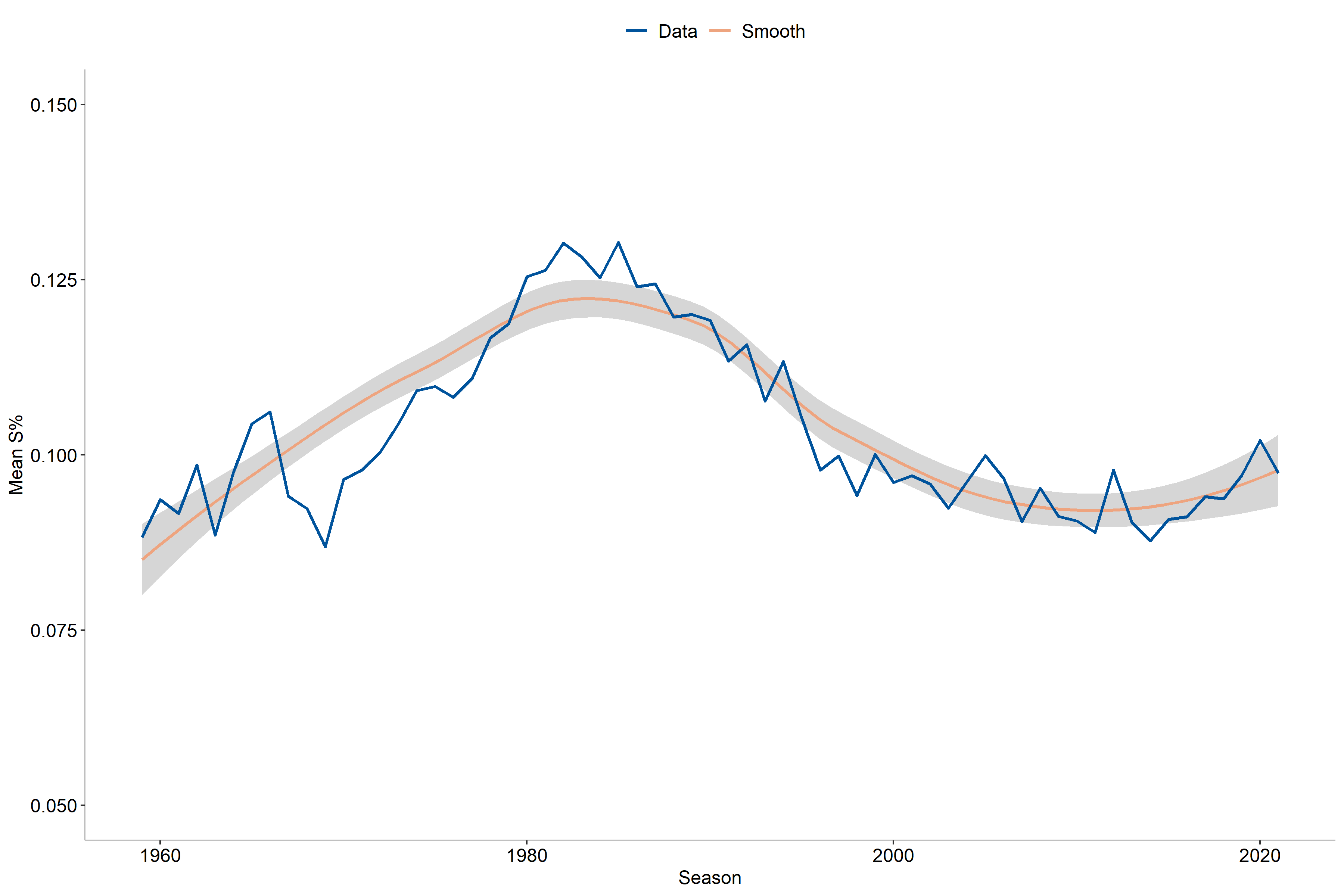
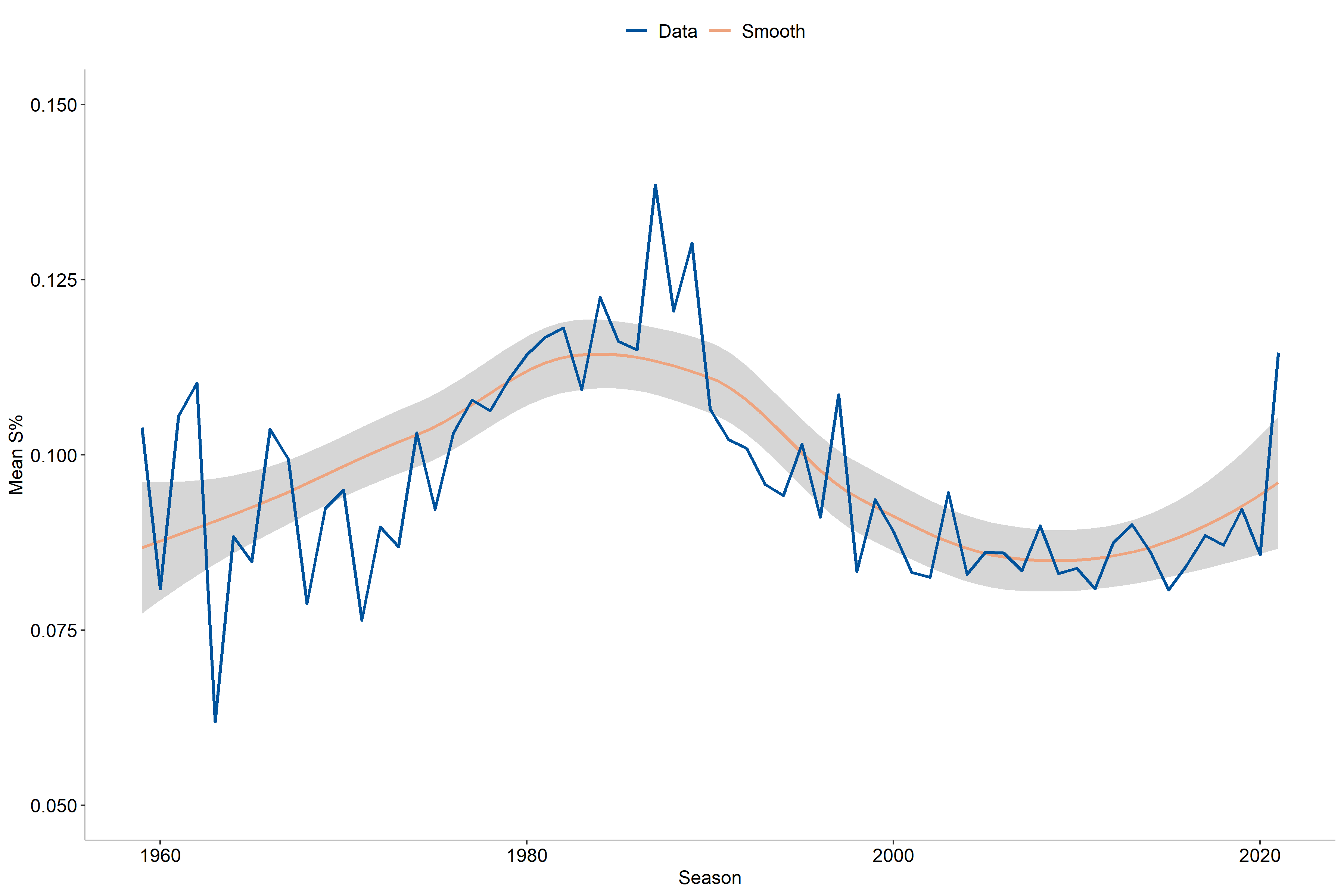
As we might have expected, the shooting percentages has indeed varied over time and does not have a linear change over time, which means we need to use a non-linear term for season. In particular, the non-linear term will be a (thin-plate) smoothing spline with a grouping by position. From the graph we also observe the highest scoring rates in the early and mid 1980’s while the lowest values were found in the 1960’s and 1970’s. Moreover, there is also a decrease near the early 2000’s that is then followed by an increase toward the modern day. When comparing single-season and career numbers, we can also note that there seems to be a higher variability for career numbers than the corresponding single-season year values. What we can be sure of however, is that the season appears to be an important factor for determining shooting percentages.
Note: The following two sections will contain some mathematical foundations for the modeling and shrinkage imposed on S%. If this is not your cup of tea feel free to skip to the results section to see the method in practice.
The Bayesics
Before introducing the method, let us first familiarize ourselves with some basics of Bayesian inference. First, we specify some notation:
$x$: Data, typically in the form of a matrix with dimension $n \times p$.
$n$: Number of observations and $p$: Number of variables.
$\theta$: A vector of (unknown) (hyper)parameters.
$\theta \vert x$: The parameters conditional of the data.
$\Pr$: Probability/probability distribution and $\propto$: Proportional to.
Here we are interested in $\theta \vert x$ and more specifically $\Pr(\theta \vert x)$, that is the probability distribution of $\theta \vert x$. To obtain this we will use Bayes’ rule:
\[\overbrace{\Pr(\theta \mid x)}^{\text{Posterior}} = \frac{\overbrace{\Pr(x \mid \theta)}^{\text{Likelihood}} \overbrace{\Pr(\theta)}^{\text{Prior}}} {\underbrace{\int_\theta \Pr(x \mid \theta) \Pr(\theta) d\theta}_{\text{Normalizing constant}} } = \frac{\Pr(x \mid \theta) \Pr(\theta)} {\Pr(x)} \propto \Pr(x \mid \theta) \Pr(\theta)\]where the three main concepts are: prior, likelihood, and posterior. The normalizing constant can also be referred to as evidence and has the role of ensuring the posterior distribution is a valid probability distribution1. Note that since $\Pr(x)$ does not depend on $\theta$ we can use the proportional form to simplify computations2.
The prior represents our prior knowledge of the phenomenon without seeing any data, while the likelihood is the probability of the observed data as a function of the data. By multiplying the prior and likelihood we can then obtain the posterior, i.e., how the parameters depend on the data.
Empirical Bayes
With the basics of Bayesian inference laid out and the task at hand we are not ready to go into the specifics of the method. The method of choice here is empirical Bayes, also called Type-II maximum likelihood, which can be seen as an approximation to the “fully” Bayesian method of a hierarchical Bayes model. Empirical Bayes differs from the other Bayesian methods in the fact that it uses data to specify it’s priors, rather than purely using prior knowledge. As a consequence, it has received some criticism as it does not allow for uncertainty in the hyperparameters of the model and subsequent estimates. However, for the case when the shrinkage is desired, such as here, it can provide reasonable results [5].
To estimate the hyperparameters under the empirical Bayes framework we can borrow a well-known technique from the realm of the frequentist, namely maximum likelihood estimation (MLE). The MLE finds the value of $\theta$ that maximizes the probability of the data $x$ given parameter(s) $\theta$, i.e.,
\[\hat{\theta} = \arg \max_{\theta} \Pr(y \mid \theta)\]where $\hat{\theta}$ is an estimate of $\theta$.
As noted previously, empirical Bayes does not account for uncertainty in its hyperparameters as they are treated as “known”. This stands in contrary to a Bayesian hierarchical model, where the prior instead would be a probability distribution, that also accounts for this uncertainty. The benefit of empirical Bayes lie in the speed of computation as well as possibility for reasonable results if the prior is too vague or do not align with the data. However, empirical Bayes can suffer from a variety of issues in different settings [3], [4], but we shall still proceed with this method as it has also been shown to work quite well for the task at hand in other sports [5].
The binomial, beta and beta-binomial distributions
The empirical Bayes method may seem abstract until now so let us now move on to how we will apply to the data in this post. A first observation is that our variable of interest, S%, is a percentage and thus is bounded between 0 and 1. Moreover, we can consider each shot as an independent3 trial with two outcomes: goal or no goal. As it turns out, this is very helpful for the next step we need to take.
Let us first turn to the actual data that we have: shots with two outcomes. In statistics and machine learning, a singular such shot is described as a Bernoulli random variable. For a random variable $Y_i$ with probability of success (= goal) $\theta$ and observed value $y_i$, the Bernoulli probability distribution is:
\[\Pr(Y_i = y_i \mid \theta) = \theta^{y_i} (1-\theta)^{1-y_i} \text{ for } y_i = \{0, 1\}.\]This means that we either score (with probability $\theta$) or don’t (with probability $1-\theta$). Unsurprisingly however, hockey players tend to shoot more than once. Fortunately for us, there is a convenient mathematical result that let us consider the sum of many independent Bernoulli trials as a binomial distribution. Consider now a random variable $Z = \sum_{i=1}^m Y_i$. This will follow a binomial distribution, which is given by:
\[\Pr(Z = k \mid m, \theta) = \binom{m}{k} \theta^k (1-\theta)^{m-k} \text{ for } k = 0, 1, \dots, m\]where $\binom{m}{k}$ is the binomial coefficient that describes how in many different ways $k$ success can be obtained from $m$ trials. This distribution then describes how we can view the likelihood of our data. But what about the prior?
The prior will in this case be placed on the probability $\theta$. In the Bayesian framework, we need to specify a distribution for this prior, and one might wonder what a reasonable choice might be? Well, in this case one such choice is the beta distribution, which is characterized by the shape parameters $\alpha$ and $\beta$. The distribution is given by:
\[f(v \mid \alpha, \beta) = \frac{1}{B(\alpha, \beta)} v^{\alpha-1} (1-v)^{\beta-1} \text{ for } v \in (0, 1), \alpha > 0, \beta > 0\]where $B(\alpha, \beta)$ is the beta function. In particular, the beta distribution has two desirable properties for us: it is bounded between 0 and 1, and it is the conjugate prior to a binomial likelihood. Brushing the mathematics aside, this basically means that for this combination of prior and likelihood, we know what form the posterior will take, which will also be a beta distribution.
However, we will need to cover one more mathematical concept before moving on. For these two distributions we can also re-write this as a compound distribution and have this be our prior. The compound distribution of a beta and binomial distribution is a beta-binomial distribution.
A beta-binomial distribution is typically described by two parameters: $\alpha$ and $\beta$, and is of the form:
\[f(v \mid \alpha, \beta, m) = \binom{m}{v} \frac{B(v + \alpha, m - v + \beta)}{B(\alpha, \beta)}.\]However, for computational purposes it is beneficial to reparameterize this distribution. That is, we instead define the parameters $\mu = \frac{\alpha}{\alpha + \beta}$ and $\sigma = \frac{1}{\alpha + \beta}$.
A particularly useful result is that the mean for a beta-binomial distribution is given by $\frac{m\alpha}{\alpha+\beta} = m\mu$. Additionally, for our posterior, which will also be a beta-binomial distribution, the posterior parameters will be
\[\alpha_1 = \alpha_0 + \text{ Goals } \quad \text{and} \quad \beta_1 = \beta_0 + \text{ Shots } - \text{ Goals}\]where ($\alpha_0$, $\beta_0$) and ($\alpha_1$, $\beta_1$) denote the prior and posterior parameters, respectively.
Finally, we will be using the set of variables described in the data section, i.e. position, number of shots, as well as a smoothing spline for season, to model both $\mu$ and $\sigma$ in the beta-binomial model. We will then do a Bayesian updating to obtain the posterior estimates.
Results
Now you may be wondering what this shrinkage actually does in practice. Before moving on to that, I would first like to highlight one alteration that has been been after the modeling, namely that of the impact of season on the estimation. As we saw previously, the shooting percentages were the highest in the 1980’s which the two left curves also detail in the figures below.
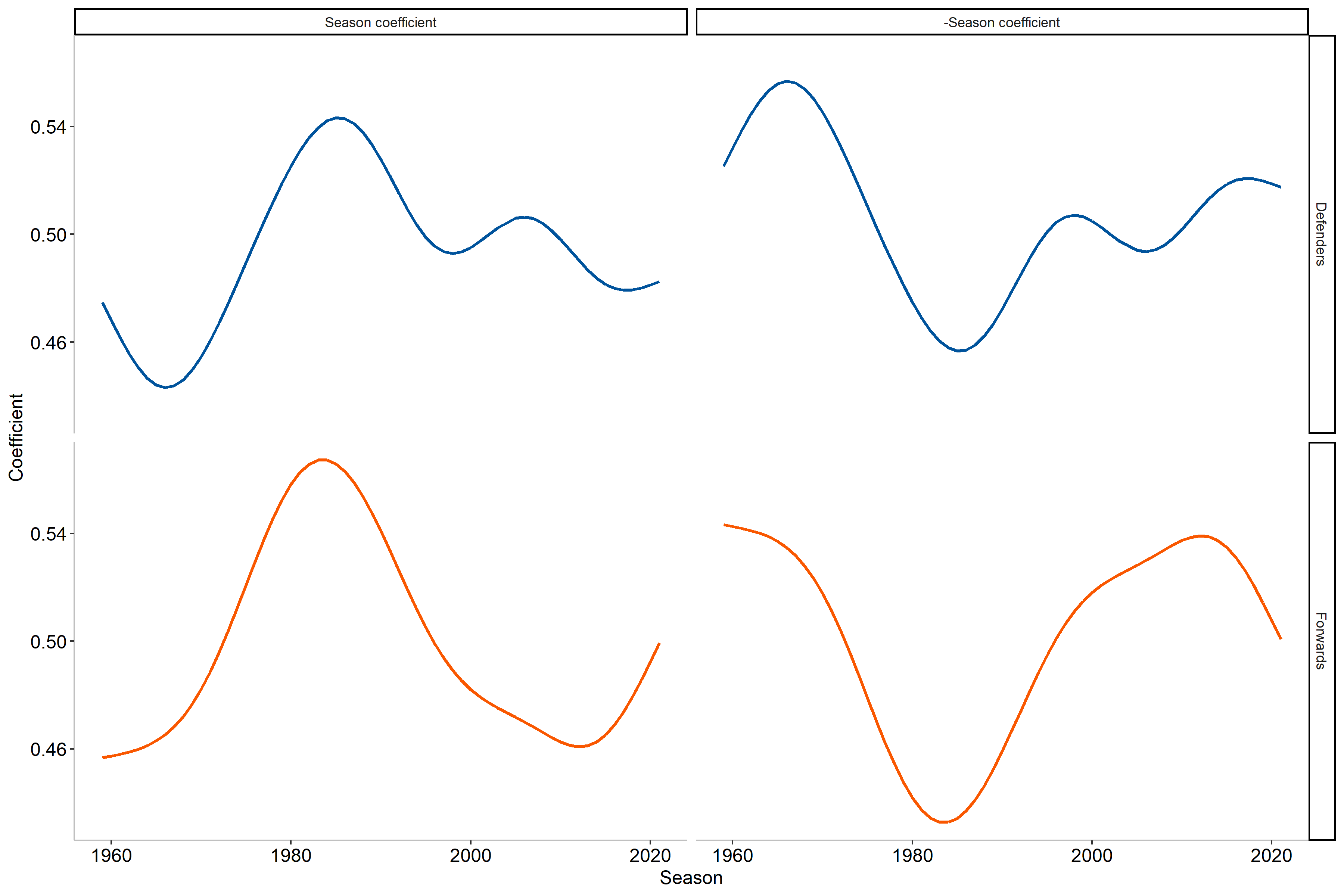
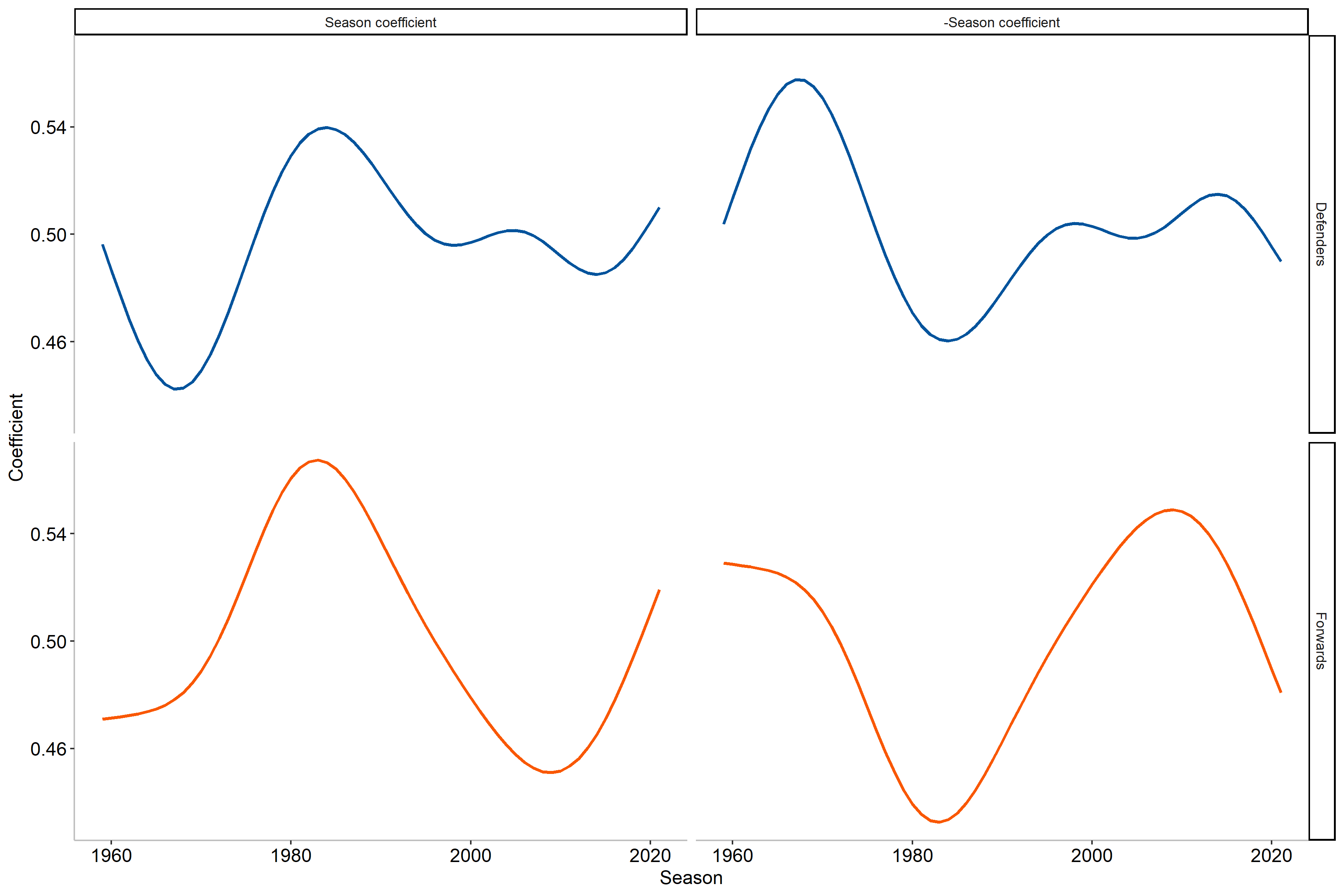
However, from the current coefficient4 we note that this means that players from that era will be shrunk less than the other eras. I would argue that we can alter this slightly, by simply taking the mirrored coefficient (negative becomes positive and vice versa). Why make such a change you ask? The reason is fairly simple: I believe that players achieving a higher shooting percentages in seasons/eras where the league average is lower is more impressive than accomplishing the same feat with a higher league average. Let us take an example to showcase this more clearly.
In the 2017-2018 NHL season William Karlsson scored 43 goals on 184 shots, a career best, which resulted in a S% of 23.37%. During this season the average S% was 9.40%. By using the original seasonal coefficient value the empirical Bayes estimation would be 17.31%, which would rank him as the 374$^\text{th}$ highest estimated S% in NHL history. However, if we were to use the adjusted coefficient the estimate instead becomes 18.48%, leading to rank 22 in NHL history. This is due to this season having a lower average S% while maintaining a reasonably large amount of shots in a single season. Let us put this into perspective by contrasting this with the 1982-1983 season of Mark Napier, where he had 40 goals on 171 shots (S% of 23.39%) when the league averaged 13.02%. Using the original coefficient he would be ranked 71$^\text{st}$ with an estimate of 19.25% while the adjusted coefficient instead estimates the S% at 16.20% and ranks him 272$^\text{nd}$. As we can see, William Karlsson had a far more effective scoring season than Mark Napier, when comparing to the league average. Consequently, we will be using the adjusted coefficient to allow players far outperforming league average to have less shrinkage.
With that being said, let us now move onward to the results!
Most effective career scorer
For efficiency reasons a minimum threshold of 1 000 career shots has been imposed to be included in the interactive table below. For the full table see here.
When it comes the the most effective career scorers the most represented era is that of the 1980’s, which should come as no surprise based on what we saw in the previous sections. Overall, Craig Simpson ranks as the most effective scorer with an estimated S% of 21.1%, while Charlie Simmer (20.6%) and Mike Bossy (20.3%) round out the top three. Notable omissions in this subset is Camille Henry (rank 5 with an estimate of 19.0%) and Sergei Makarov (rank 7 with an estimate of 18.7%). For some of the most prolific goal-scorers in NHL history the ranks are Wayne Gretzky (26$^\text{th}$), Mario Lemieux (8$^\text{th}$), Jaromir Jagr (297$^\text{th}$), Brett Hull (120$^\text{th}$), and Alexander Ovechkin (436$^\text{th}$). Among defenders the most effective career scorer is Denis Potvin, although he only ranks 2670$^\text{th}$.
Most effective single-season scorer
For efficiency reasons a minimum threshold of 150 single-season shots has been imposed to be included in the table. For the full table see here.
Focusing on single-season numbers instead, we again see some familiar players from the career scoring results. However, this time the top players tend to belong to the Edmonton Oilers in the mid 1980’s, a team lead by Wayne Gretzky to four Stanley cups. Gretzky also had the second and third most effective scoring seasons in NHL history, trailing only Mario Lemieux’s 1988-1989 campaign. Beside Gretzky, we also find his teammates Jari Kurri and Craig Simpson. Yet again we can also see that the 1980’s is the era with highest estimated shooting percentages, although some players break this dominance. For instance, William Karlsson’s 2017-2018 season ranks 22$^\text{nd}$, the 1971-1972 campaign of Jean Ratelle ranking 17$^\text{th}$, Johnny Bucyk’s 1970-1971 season ranks 20$^\text{th}$, and the 2011-2012 season of Steven Stampkos ranks 25$^\text{th}$. In addition, Camille Henry’s 1962-1963 season has rank 14 although he took 139 and thus is not shown in this table. Among defenders, Paul Coffey and Bobby Orr share the top five most effective scoring seasons among themselves, with Coffey at rank 1 and 3, while Orr takes 2, 4, and 5. Their overall ranks are however quite low, the highest being 16585$^\text{th}$.
Acknowledgements
This post draws inspiration from the work by David Robinson and his book “Introduction to Empirical Bayes: Examples from Baseball Statistics”.
References
[1] Jensen, S. T., McShane, B. B., & Wyner, A. J. (2009). Hierarchical Bayesian modeling of hitting performance in baseball. Bayesian Analysis, 4(4), 631-652.
[2] Albert, J., & Birnbaum, P. (2009). Comment on Article by Jensen et al. Bayesian Analysis, 4(4), 653-660.
[3] Liu, S., Kuppens, P., & Bringmann, L. (2021). On the use of empirical Bayes estimates as measures of individual traits. Assessment, 28(3), 845-857.
[4] Scott, J. G., & Berger, J. O. (2010). Bayes and empirical-Bayes multiplicity adjustment in the variable-selection problem. The Annals of Statistics, 2587-2619.
[5] Robinson, D. (2017). Introduction to Empirical Bayes: Examples from Baseball Statistics. E-book.
-
In order for a probability distribution to be valid it needs to satisfy two requirements: the probability for each value in its support need to be bounded between 0 and 1, and the sum of all probabilities must equal 1. Specifically, we have $\Pr(a \leq X \leq b) = \int_{a}^{b} f_X(x) dx$ with $f_X$ as a non-negative Lebesgue-integrable function. When integrating this we obtain the value 1. ↩
-
In many cases, the integral in the denominator is intractable or in general computationally expensive. As such, to make computations much faster or even feasible, we use the proportionality property to obtain a result and perform inference. Do note however, that in some cases the normalizing constant is required as it is what ensures that we have a valid probability distribution. ↩
-
In reality, this is not entire true as rebounded shots are dependent on a previous shot being taken, as well as tip-ins amongst other things. However, this assumption simplifies computation a great deal and will be treated as reasonable throughout this post. ↩
-
Coefficient is the value that describes the relationship between a variable and the target. ↩


